2.6 Filtering Basics

Sensors are prone to physical and electrical interference from their environment which can obscure input measurements. Noise, or the unwanted disturbances to the true input values, can often be statistically modeled and diminished with specific filters.

Gaussian Noise

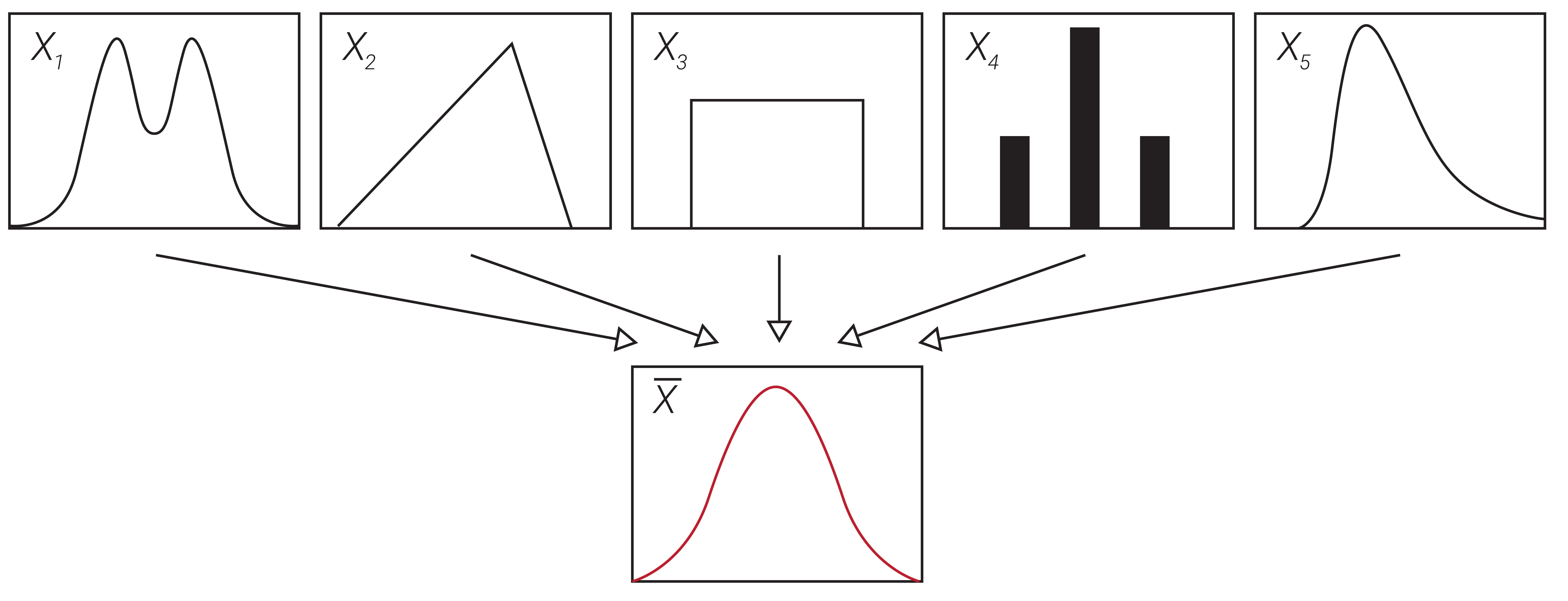
In probability theory, a distribution termed the Gaussian distribution has found many applications in describing real-world events. This distribution is also known as a normal distribution or bell curve due to its shape, as seen in Figure 2.8a. The central limit theorem states that as independent random variables are summed, the result tends to approach a Gaussian distribution, even if the variables themselves are non-Gaussian, as illustrated in Figure 2.8b. As variables (or error sources) are combined, the result ends up resembling the normal distribution, making it a reasonable approximation for most real-world systems.

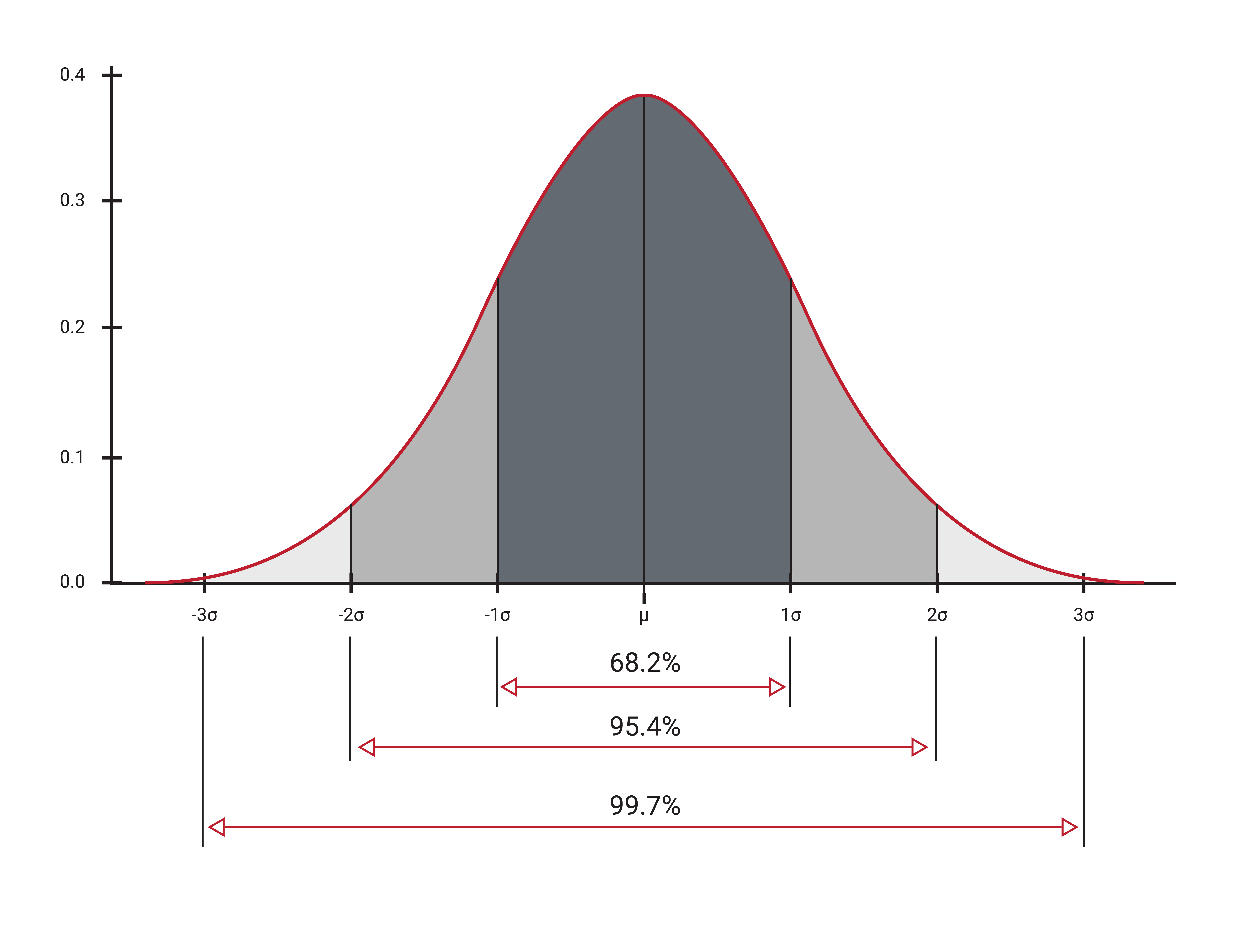
Values less than one standard deviation ($1\text{-}\sigma$), from the mean account for 68.2 % of all samples while two and three standard deviations ($2\text{-}\sigma$, $3\text{-}\sigma$) contain 95.4 % and 99.7 % of all samples, respectively. Gaussian noise is noise that occurs within a Gaussian or normal distribution. It is assumed that Gaussian noise is zero-mean, with uncorrelated samples independent of previous values.

Standard Deviation, RMS, and Variance

When working with data sets, it can be useful to know the variation of a set of measurements. Variance, standard deviation, and the root-mean-square (RMS) are different ways to quantify this variation. The variance is a measure of the variation of a set of measurements with respect to themselves and can be described using Equation \ref{eq:fbvar}, where $\sigma^2$ is the variance, $N$ is the total number of measurements in a data set, $x_i$ is the $i^{\text{th}}$ measurement in the data set, and $\mu$ is the mean of the set of measurements.

\begin{equation} \label{eq:fbvar} \sigma^2 = \frac{1}{N-1}\sum_{i=1}^N (x_i-\mu)^2 \end{equation}

Standard deviation is another way to describe the variation of a set of measurements with respect to themselves and is given by Equation \ref{eq:fbsd}.

\begin{equation}\label{eq:fbsd} \sigma = \sqrt{\frac{1}{N}\sum_{i=1}^N (x_i-\mu)^2}\end{equation}

From these equations, it can be seen that the standard deviation is simply the square root of the variance. When describing the variation in a set of measurements with respect to themselves, it is typically easier to visualize how the standard deviation relates to the original data set (since they have the same units) and is much more commonly used to describe the variation than the variance.

The root-mean-square (RMS) quantity is often a term that is used interchangeably with standard deviation, although these two characteristics have quite different meanings. RMS describes the variation of measurements with respect to the true value, rather than with respect to their mean, and can be found using Equation \ref{eq:fbrms}, where $x_t$ is the true value that the measurements should read. If a quantity is unbiased---has zero-mean error---then RMS and standard deviation are indeed equivalent.

\begin{equation} \label{eq:fbrms}\mbox{RMS} = \sqrt{\frac{1}{N-1}\sum_{i=1}^N(x_i-x_t)^2}\end{equation}

Digital Filters

As microprocessor speeds have increased, it has become possible to process signals in software and apply digital filters to modify the input measurements. Digital filtering can be used in place of analog filtering to collect the desired data while removing noise. While this lowers the required circuit board component count, it does require additional software to handle the algorithms involved. Digital filters also have the advantage of being able to be adjusted within software, and can achieve filtering that would be difficult using analog components.

IIR Filter vs FIR Filter

The two main types of digital filters are known as infinite-impulse response (IIR) filters and finite-impulse response (FIR) filters. As shown in the most basic IIR filter in Equation \ref{eq:fbiir}, an IIR filter uses feedback in the form of the previous filtered result in filtering a measurement, so any anomaly that occurs in the data will always have some component left in the current value.

\begin{equation} \label{eq:fbiir} Y_k = \alpha Y_{k-1}+(1-\alpha)X_k\end{equation}

In this equation, the previous filtered result, $Y_{k-1}$, is the feedback term, $X_k$ is the current measurement, and $\alpha$ is a multiplier less than 1. Larger values of $\alpha$ produce a smoother filtered result, while smaller values provide a more responsive (but noisier) output. IIR filters are easier and more efficient to implement in real-time since not much data buffering is required, but are less capable than FIR filters.

An FIR filter, the most common of which is referred to as a moving average filter or boxcar filter, uses previous measurements, but not previous outputs, in filtering a new measurement. These filters are always stable and can implement any type of filter response imaginable with enough previous values. A simple N-element low-pass boxcar filter can be implemented using Equation \ref{eq:fbfir}, where $N$ is the number of samples used in the filter.

\begin{equation}\label{eq:fbfir} Y_k = \frac{1}{N}(X_k + X_{k-1} + ... +X_{k-N+1})\end{equation}

Coefficients can also be applied to affect the frequency response of the filter. Additionally, FIR filters cause a linear phase shift for all frequencies, a useful property that can't be accomplished with analog or IIR filters. While this type of filter is generally considered more powerful, it does require a buffer to store previous values and can be more complex and time-consuming to implement than IIR filters.

Low-Pass, High-Pass, Band-Pass and Notch Filters

Depending on the frequency response desired, filters can be designed to pass or attenuate a range of different frequencies. Filters designed to pass low frequency signals while rejecting high frequency signals are called low-pass filters. High-pass filters reject low frequency signals and pass high frequency ones. Band-pass filters only allow signals in a certain range and reject all others, while notch or band-stop filters reject signals in a certain range and pass values outside of this range. The effect of each of these filters is shown in Figure 2.9.

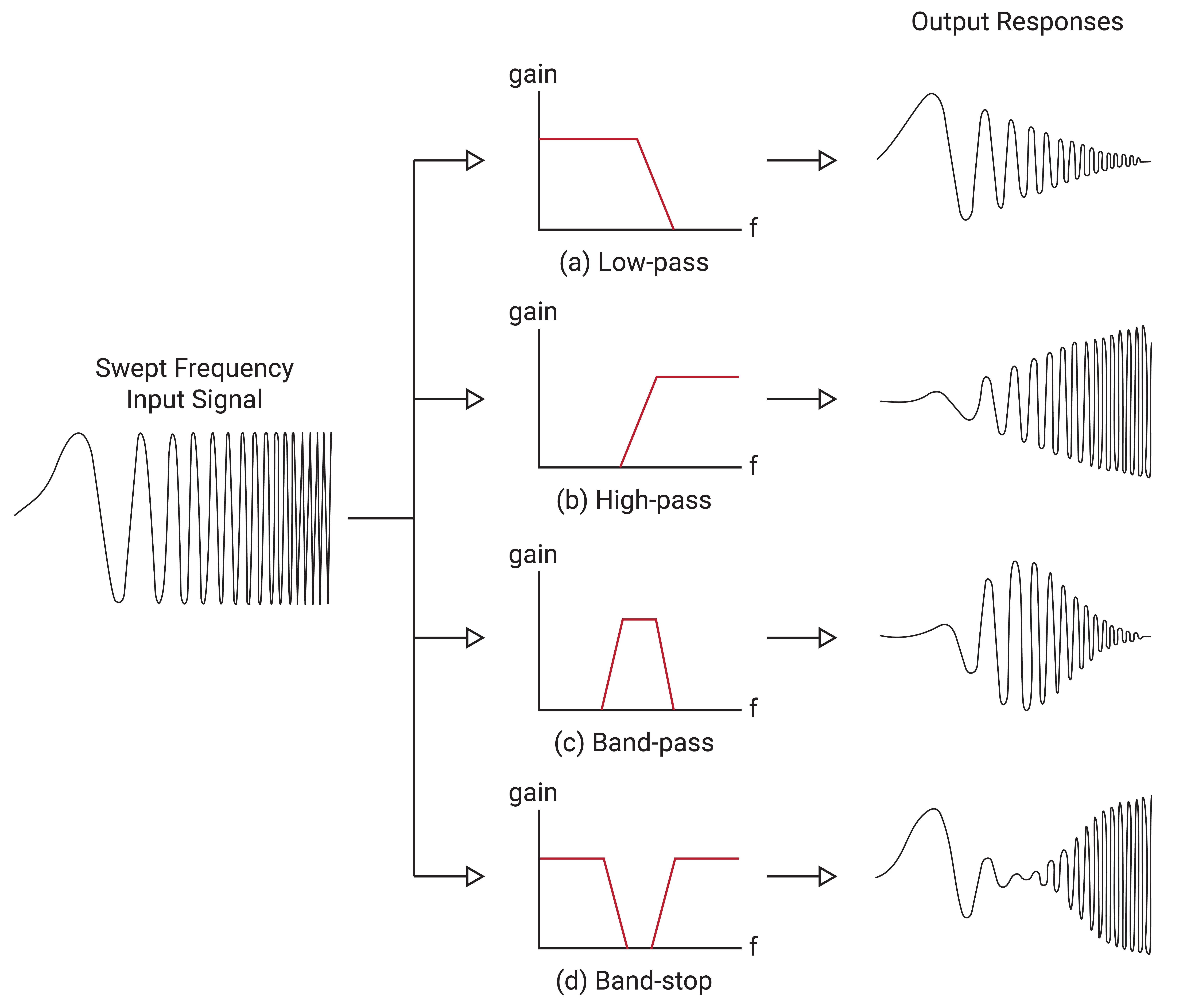
From Figure 2.9, it can be seen that as the signal is swept from a low frequency to a higher frequency, the amplitude of the output response varies depending on the type of filter it passes through. Examples of filter use include applying a high-pass filter to a gyroscope to remove bias and a low-pass filter to an accelerometer to remove vibrations. Band pass filters can remove noise in signal transmission applications and band stop filters can remove specific troublesome frequencies.

Phase Lag vs Smoothing

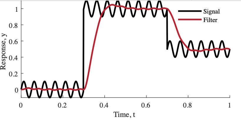
When a digital filter is applied to a measurement, a delay known as phase lag is introduced between the input signal and the filtered signal. As shown in Figure 2.10, the filtered output is smoother than the original signal and contains less change between successive data points, but there is a delayed response when sudden state changes occur in the original signal. Finding the best digital filter for an application requires making an acceptable trade-off between smoothness and phase lag.

Complementary Filters

In certain situations, data from multiple sources can be combined using different filter types to determine a state, a simple method known as complementary filtering. For example, a gyroscope works best with high-pass filtering (HPF) to remove the gyro bias from the data, while an accelerometer is best when a low-pass filter (LPF) removes vibrations and other high frequency effects. As illustrated in Figure 2.11, the pitch/roll of a system can be determined by combining the filtered results of these two sensors.

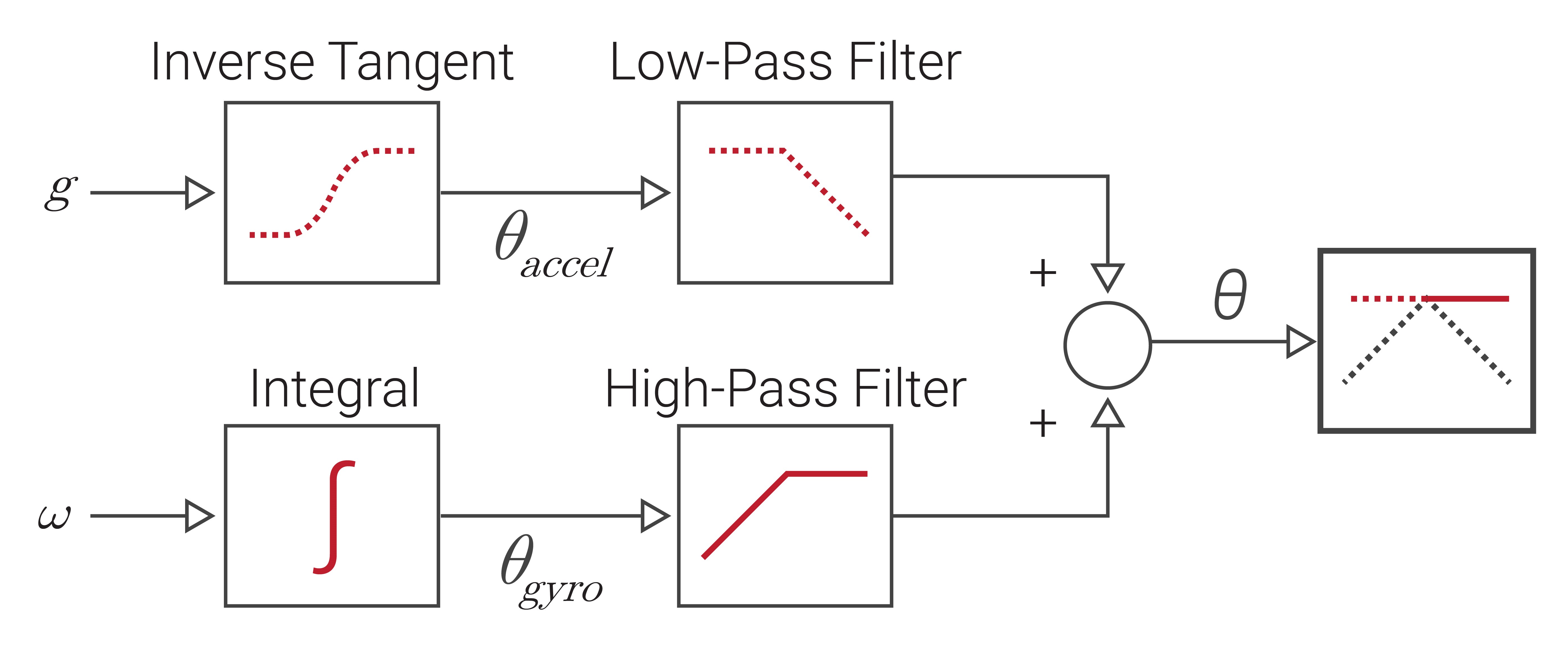
Mathematically, this is accomplished using Equation \ref{eq:fbcf}, in which $\theta$ is calculated the pitch or roll angle, $\omega$ is the angular rate measured by the gyro, and $\theta_{accel}$ is the pitch/roll angle derived from the accelerometer data (see Section 1.6).

\begin{equation} \label{eq:fbcf} \theta_{k+1} = \alpha(\theta_k + \omega\Delta t) + (1-\alpha) \theta_{accel}\end{equation}

The weight, $\alpha$, can be applied to adjust the contribution from each sensor and gives the system a complementary nature. The simplicity of the complementary filter is both its greatest strength and its greatest weakness. As discussed in Section 2.8, more advanced filters, like Kalman filters, can achieve substantially improved performance, but at the cost of computational complexity.