2.3 Attitude Representations

An attitude representation is often defined as a set of coordinates that describe the orientation of a given reference frame with respect to a second reference frame. Defining the rotational orientation of a rigid body requires a minimum of three parameters, however, many attitude representations utilize more than three parameters in defining the orientation. While there are numerous attitude representations that can be used to define the orientation of a system, some of the more common representations include direction cosine matrices (DCM), Euler angles, and quaternions.

Direction Cosine Matrix

The direction cosine matrix (DCM) is one of the many ways to mathematically represent an object's orientation and utilizes nine parameters. Each of these parameters are referred to as the direction cosine values between an initial reference frame and a second reference frame. Consider two reference frames $\mathcal{B}$ and $\mathcal{N}$, where $\mathcal{B}$ represents a body frame and $\mathcal{N}$ is defined as the inertial reference frame. Since $\mathcal{B}$ and $\mathcal{N}$ are reference frames, both are defined by a set of three orthonormal vectors that make up a right-handed system. These vectors can be expressed as $\{\hat{\boldsymbol{n}}\}$ and $\{\hat{\boldsymbol{b}}\}$, as described in Equation \ref{eq:dcmn}.

\begin{equation} \label{eq:dcmn}\{\hat{\boldsymbol{n}}\} = \left\{\begin{matrix} \hat{\boldsymbol{n}}_1\\\hat{\boldsymbol{n}}_2\\\hat{\boldsymbol{n}}_3\end{matrix}\right\} \quad \{\hat{\boldsymbol{b}}\} = \left\{\begin{matrix} \hat{\boldsymbol{b}}_1\\\hat{\boldsymbol{b}}_2\\\hat{\boldsymbol{b}}_3\end{matrix}\right\}\end{equation}

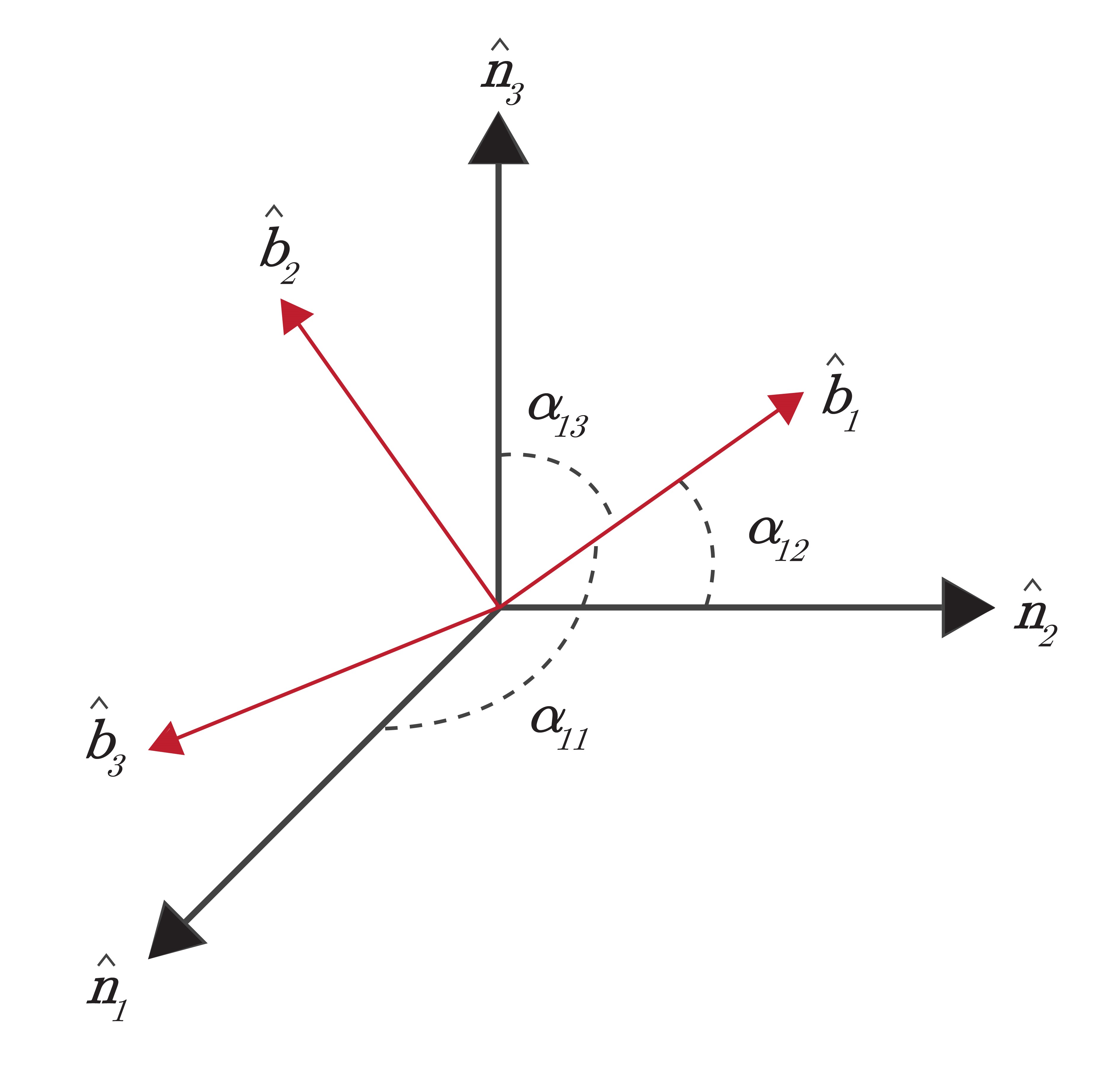
As shown in Figure 2.4, the vector $\hat{\boldsymbol{b}}_1$ creates an angle $\alpha$ with each of the vectors $\hat{\boldsymbol{n}}_1$, $\hat{\boldsymbol{n}}_2$, and $\hat{\boldsymbol{n}}_3$. In order to determine the direction cosine values of $\hat{\boldsymbol{b}}_1$ with respect to the $\mathcal{N}$ reference frame, the cosine of each of these angles is taken. The same follows for the other two vectors $\hat{\boldsymbol{b}}_2$ and $\hat{\boldsymbol{b}}_3$. Each of the unit vectors of $\{\hat{\boldsymbol{b}}\}$ can be represented in terms of the unit vectors of $\{\hat{\boldsymbol{n}}\}$ as shown in Equation \ref{eq:ardcm}.

\begin{equation} \begin{split}\hat{\boldsymbol{b}}_1 &= \cos\,\alpha_{11}\:\hat{\boldsymbol{n}}_1 + \cos\,\alpha_{12}\:\hat{\boldsymbol{n}}_2 + \cos\,\alpha_{13}\:\hat{\boldsymbol{n}}_3\\\hat{\boldsymbol{b}}_2 &= \cos\,\alpha_{21}\:\hat{\boldsymbol{n}}_1 + \cos\,\alpha_{22}\:\hat{\boldsymbol{n}}_2 + \cos\,\alpha_{23}\:\hat{\boldsymbol{n}}_3\\\hat{\boldsymbol{b}}_3 &= \cos\,\alpha_{31}\:\hat{\boldsymbol{n}}_1 + \cos\,\alpha_{32}\:\hat{\boldsymbol{n}}_2 + \cos\,\alpha_{33}\:\hat{\boldsymbol{n}}_3\end{split}\label{eq:ardcm}\end{equation}

These three equations can also be expressed in matrix form as shown in Equation \ref{eq:ardcmmbn}.

\begin{equation} \label{eq:ardcmmbn}\{\hat{\boldsymbol{b}}\} = \left[\begin{matrix}\cos\,\alpha_{11}&\cos\,\alpha_{12}&\cos\,\alpha_{13}\\\cos\,\alpha_{21}&\cos\,\alpha_{22}&\cos\,\alpha_{23}\\\cos\,\alpha_{31}&\cos\,\alpha_{32}&\cos\,\alpha_{33}\end{matrix}\right]\{\hat{\boldsymbol{n}}\}= \left[C_{\mathcal{B}\mathcal{N}}\right]\{\hat{\boldsymbol{n}}\}\end{equation}

The quantity $C_{\mathcal{B}\mathcal{N}}$ is referred to as the DCM of $\mathcal{B}$ with respect to $\mathcal{N}$. Similarly, the unit vectors of $\{\hat{\boldsymbol{n}}\}$ can be projected onto the unit vectors of $\{\hat{\boldsymbol{b}}\}$ using Equation \ref{eq:dcmmnb}.

\begin{equation} \label{eq:dcmmnb}\{\hat{\boldsymbol{n}}\} = \left[\begin{matrix}\cos\,\alpha_{11}&\cos\,\alpha_{21}&\cos\,\alpha_{31}\\\cos\,\alpha_{12}&\cos\,\alpha_{22}&\cos\,\alpha_{32}\\\cos\,\alpha_{13}&\cos\,\alpha_{23}&\cos\,\alpha_{33}\end{matrix}\right]\{\hat{\boldsymbol{b}}\} = \left[C_{\mathcal{N}\mathcal{B}}\right]\{\hat{\boldsymbol{b}}\} = \left[C_{\mathcal{B}\mathcal{N}}\right]^{\intercal}\{\hat{\boldsymbol{b}}\}\end{equation}

This simple method can also be used to transform vectors from one reference frame into another. Consider a vector $\boldsymbol{v}$ that has its components in the $\mathcal{N}$ reference frame but needs to be described in the $\mathcal{B}$ reference frame. This can be accomplished using Equation \ref{eq:dcmv}. Likewise, a vector which has its components in the $\mathcal{B}$ reference frame can be transformed into the $\mathcal{N}$ reference frame with Equation \ref{eq:dcmvnb}.

\begin{equation} \label{eq:dcmv}^\mathcal{B}\boldsymbol{v} = \left[C_{\mathcal{B}\mathcal{N}}\right]{}^\mathcal{N}\boldsymbol{v}\end{equation}

\begin{equation} \label{eq:dcmvnb}^\mathcal{N}\boldsymbol{v} = \left[C_{\mathcal{B}\mathcal{N}}\right]^{\intercal}{}^\mathcal{B}\boldsymbol{v}\end{equation}

There are a few properties of the DCM that make it a unique method for representing an object's attitude. For example, the norm of each row and column of the DCM must be equal to +1. In addition, the DCM is orthogonal and more specifically, orthonormal. This means that the product of $[C_{\mathcal{B}\mathcal{N}}]$ and the transpose of $[C_{\mathcal{B}\mathcal{N}}]$ results in the identity matrix as shown in Equation \ref{eq:dcmi}.

\begin{equation} \label{eq:dcmi}\left[C_{\mathcal{B}\mathcal{N}}\right]\left[C_{\mathcal{B}\mathcal{N}}\right]^{\intercal} = \left[C_{\mathcal{B}\mathcal{N}}\right]^{\intercal}\left[C_{\mathcal{B}\mathcal{N}}\right] = \left[I_{3\times3}\right]\end{equation}

Furthermore, this means that the transpose of $[C]$ is equal to its inverse:

\begin{equation}\left[C_{\mathcal{B}\mathcal{N}}\right]^{\intercal}= \left[C_{\mathcal{B}\mathcal{N}}\right]^{-1}= \left[C_{\mathcal{N}\mathcal{B}}\right]\end{equation}

One final DCM property to note is that of the determinant. For a right-handed system, the determinant of the DCM must be equal to +1.

\begin{equation}\det\left[{C_\mathcal{BN}}\right] = +1\end{equation}

While the direction cosine matrix is an important and commonly used method for representing an object's attitude, there is one major drawback to this approach. The DCM utilizes nine parameters to describe an orientation. Since only three parameters are required, six of the DCM values are redundant. Due to this, the DCM is hardly ever used to keep track of attitude in real time and is instead used primarily to project vectors to different reference frames.

Euler Angles (Yaw-Pitch-Roll)

The orientation of a rigid body can also be described by three successive rotations about a set of intermediary axes, which transform the body from an inertial reference frame into the body frame. These three rotations are the most frequently used method for representing an object's attitude and are known as the Euler angles.

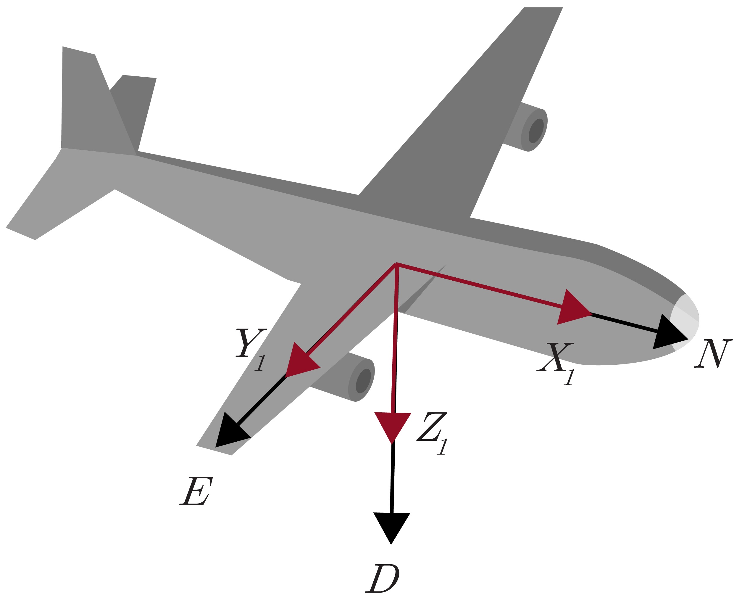
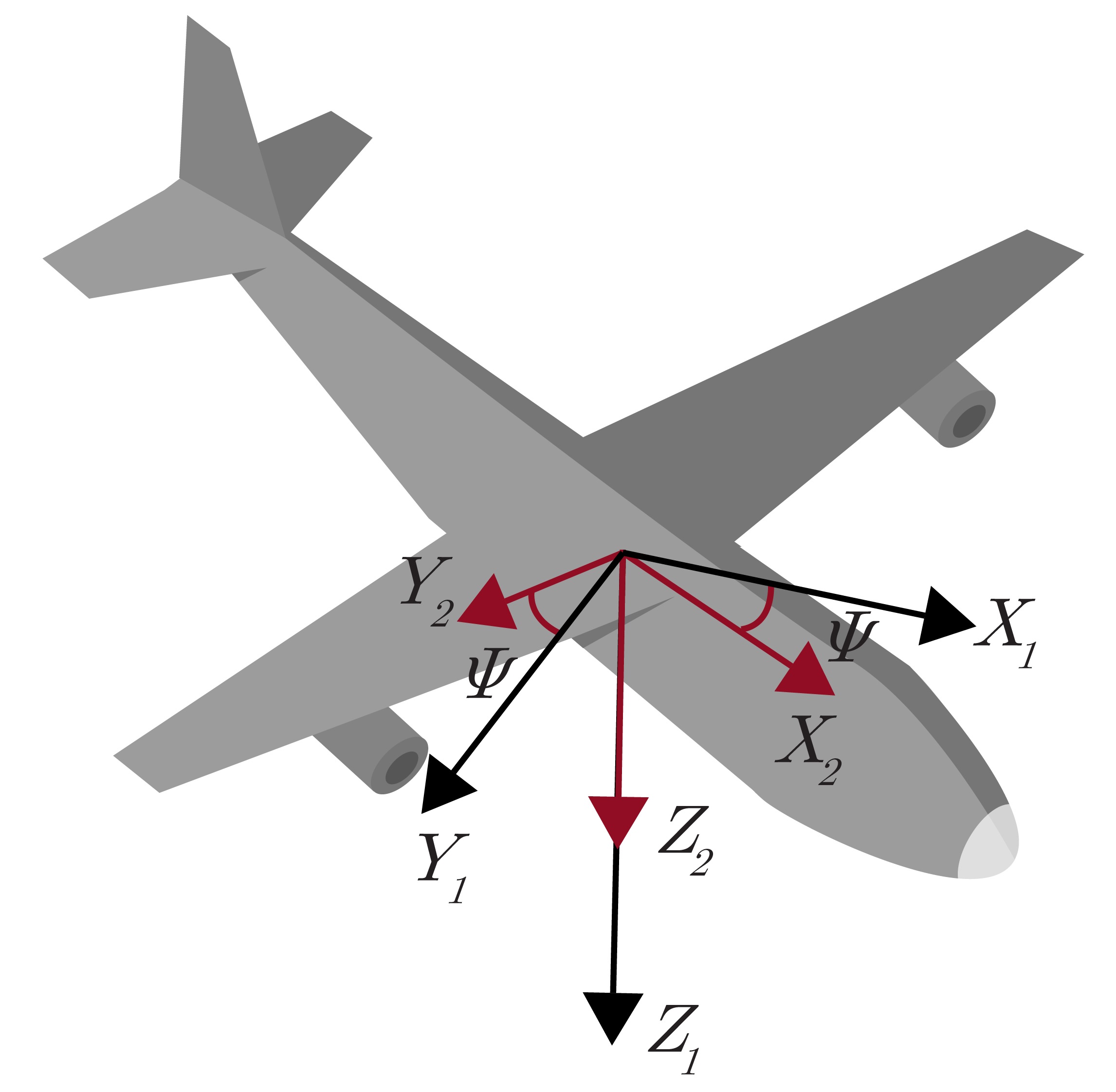
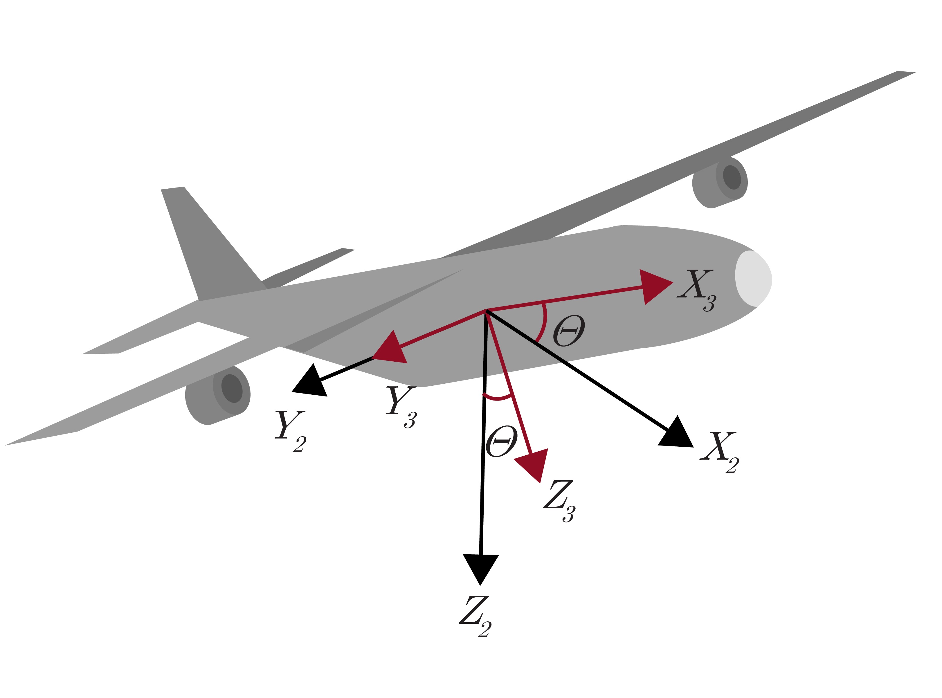
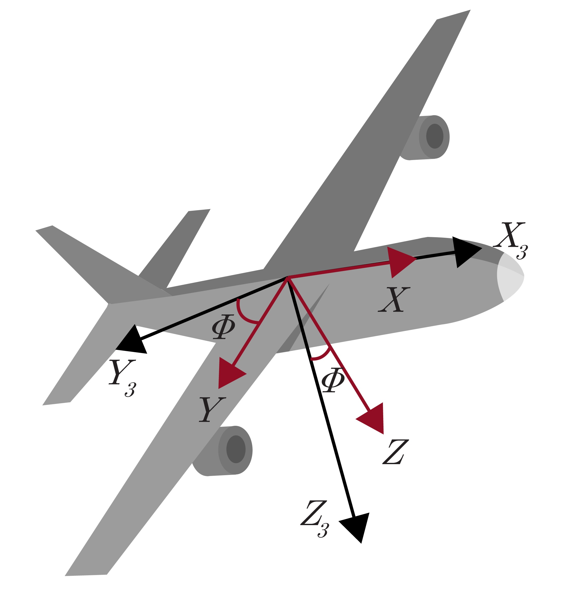
There are many different combinations of Euler angles, however, the (3-2-1) set of Euler angles corresponding to yaw-pitch-roll ($\psi $-$\theta$-$\phi$) is considered to be the standard, especially in terrestrial applications. These rotations are applied sequentially in a particular order, with each rotation specified about the specified body frame axis as it exists following the previous rotations. Figure 2.5a shows the body frame and NED frame initially aligned. Figure 2.5b shows the yaw rotation around the $Z_1$-axis. This is followed in Figure 2.5c by the pitch rotation about the new $Y_2$-axis. Finally, there is a roll rotation about the new $X_3$-axis in Figure 2.5d to achieve the final orientation of the aircraft.

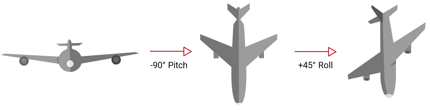
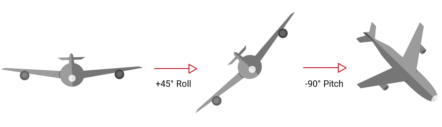
The order of these rotations is important, as a (3-2-1) set of Euler angles corresponding to yaw-pitch-roll can result in a much different orientation than applying those same angles in a (1-2-3) sequence of roll-pitch-yaw. As an example, Figure 2.6 shows the difference between applying a -90° pitch, followed by a 45° roll (Fig. 2.6a), and applying a 45° roll, followed by a -90° pitch (Fig. 2.6b). The end orientation of the aircraft is very different!

It is important to note that this order does not have as much of an effect when the angles are small. This makes Euler angles particularly easy to visualize and therefore are the most commonly used attitude representation.

While this seems to be an ideal way to represent attitude there is one major drawback to this method: every set of Euler angles has at least one geometric singularity, often referred to as gimbal lock. This means that at a specific orientation, two of the axes become ambiguous. For example, in the standard set of (3-2-1) Euler angles, this singularity exists when the pitch is $\pm$90°. In this case, the yaw and roll perform the same operation, as a yaw angle of 20° and a roll angle of 0° results in an orientation identical to that of a yaw angle of 0° and a roll angle of 20°. As a result, Euler angles must be used with caution, especially in applications that deal with angles close to the singularity points.

Euler's Principal Rotation Theorem

Euler's principal rotation theorem states that any rigid body or reference frame can be taken from an initial orientation to a final orientation via a single rigid body rotation about a principal axis, $\hat{\boldsymbol{e}}$, through a principal angle, $\phi$. Simply put, any arbitrary orientation can be described by a single unit vector and a single angle, as shown in Figure 2.7.

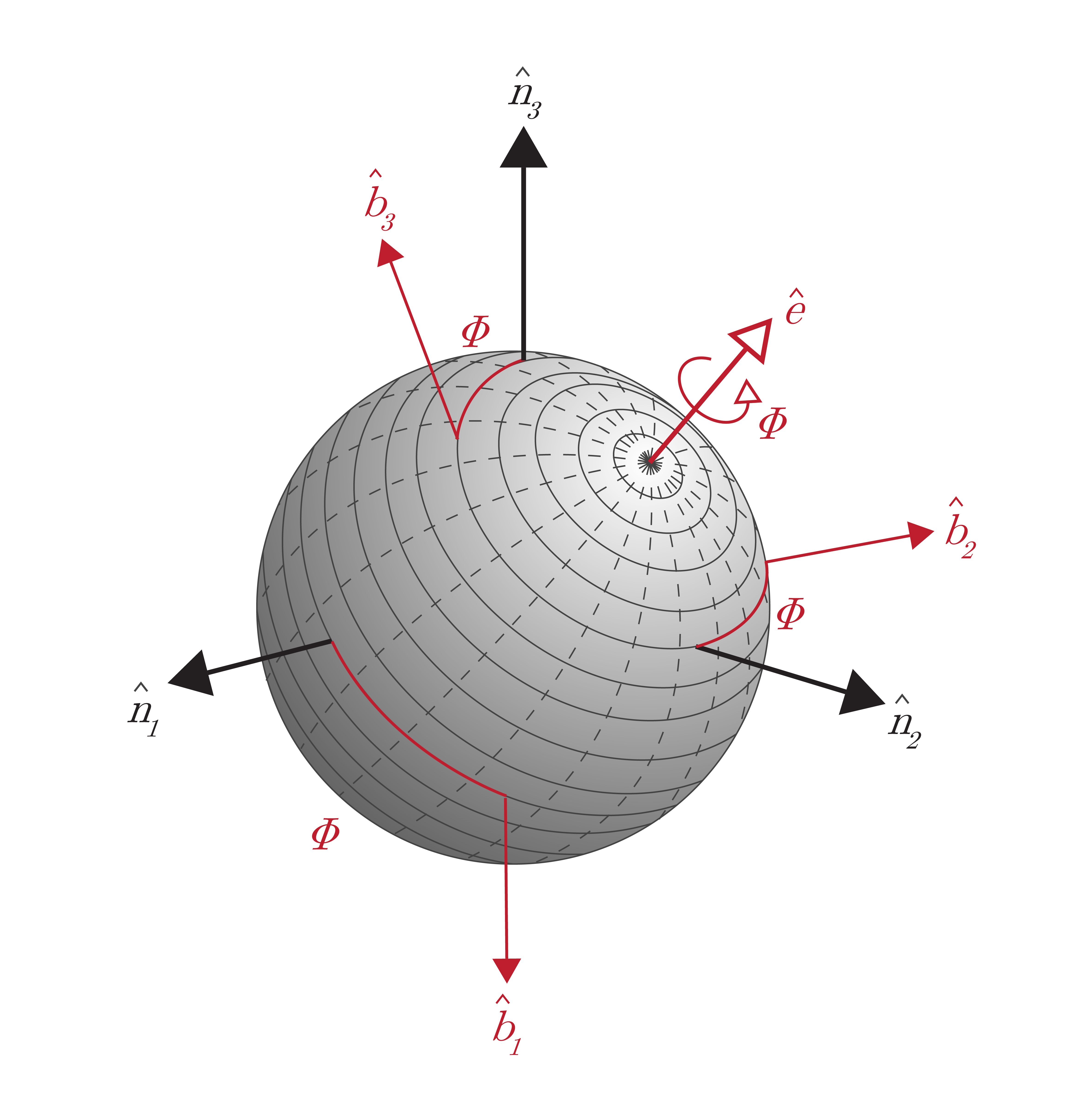
The principal axis defines the direction of rotation while the principal angle describes the amount of rotation about this axis from the initial attitude to the final attitude. This principal rotation theorem is valid for any rotation and the principal angle is useful as a scalar measure of the difference between two attitudes, such as the error between the measured attitude and the truth. Furthermore, the principal axis and principal angle form the basis for defining many other attitude representations.

Quaternion

A quaternion is an attitude representation that uses a normalized four-dimensional vector to describe a three-dimensional orientation. This approach is based upon Euler's principal rotation and consists of a scalar term $q_s$ and a vector term $q_v$ as shown in Equation \ref{eq:quat}.

\begin{equation} \begin{split}\boldsymbol{q}_v &= \hat{\boldsymbol{e}}\sin\frac{\strut\phi}{\strut2} = \left[\begin{matrix}e_1\sin\frac{\strut\phi}{\strut2}\\e_2\sin\frac{\strut\phi}{\strut2}\\e_3\sin\frac{\strut\phi}{\strut2}\end{matrix}\right]\\q_s &= \cos\frac{\phi}{2}\end{split}\label{eq:quat}\end{equation}

Typically, the quaternion is represented by a single four-element vector. It is important to note that there is no agreed upon order for that four-element vector, so it is important to be clear whether a system or equation is assuming the scalar term last (Eq. \ref{eq:quatvs}) or first (Eq. \ref{eq:quatsv}). VectorNav sensors and documentation utilize the scalar term last representation.

\begin{equation} \label{eq:quatvs}\boldsymbol{q} = \left[\begin{matrix}\boldsymbol{q}_v\\q_s\end{matrix}\right]\end{equation}

\begin{equation} \label{eq:quatsv}\boldsymbol{q'} = \left[\begin{matrix}q_s\\\boldsymbol{q}_v\end{matrix}\right]\end{equation}

The quaternion is advantageous as it circumvents the singularity problem of Euler angles by adding an additional parameter, creating an over-defined attitude representation. However, this does create an over-defined attitude representation and requires the constraint that the norm of the quaternion be equal to one. Note also that there is an ambiguity when representing an attitude by a quaternion, because $\boldsymbol{q}\equiv-\boldsymbol{q}$.