2.8 Kalman Filter

Originally developed in 1960 by R.E. Kalman, the Kalman filter provides an optimal estimate of how a system is going to change given noisy measurements and imperfect knowledge about the system. The Kalman filter is similar to least squares in many ways, but is a sequential estimation process, rather than a batch one. The standard Kalman filter is designed mainly for use in linear systems and is widely used in many different industries, including numerous navigation applications.

State Vector and State Covariance Matrix

As discussed in Section 2.7, many applications contain a number of different sensors that can be used to determine various parameters of interest in a system, commonly referred to as states. Unfortunately, a sensor is typically not able to provide a direct measurement of a state, but rather yields a noisy measurement containing some uncertainty that indirectly provides some information about one or more states.

The standard Kalman filter was developed to combine and process all available information about a linear dynamic system, both its dynamics model and any measurements, into an optimal estimate of the state. This state estimate is optimal in the sense that the variance is minimized, assuming that the measurement errors in the system are Gaussian and zero-mean. To help explain how a standard Kalman filter works, consider an aircraft that needs to track its position and velocity as it flies to its destination. The estimated position ($p$) and velocity ($v$) form the estimated state vector, $\hat{\boldsymbol{x}}$:

\begin{equation}\label{eq:kfstate} \boldsymbol{x} = \begin{bmatrix}p\\v\end{bmatrix}\end{equation}

The key to a Kalman filter is that in addition to maintaining an estimate of the state, it also tracks an estimate of the uncertainty associated with that state---recognizing that the position and velocity estimates are never perfectly known. This uncertainty can be represented by a matrix known as the state covariance matrix, $P$. The state covariance matrix consists of the variances associated with each of the state estimates as well as the correlation between the errors in the state estimates. The covariance matrix can be graphically represented by n-D ellipsoids (where $n$ is the number of states), where a particular ellipsoid maps to the $1\text{-}\sigma$, $2\text{-}\sigma$, or $3\text{-}\sigma$ uncertainty bounds.

In this particular system, $\sigma_{p}^{2}$ and $\sigma_{v}^{2}$ in Equation \ref{eq:kf_P} are the variances associated with each of the state estimates and $\gamma_{pv}$ is a value between 0 and 1, representing the correlation between the position and velocity errors.

\begin{equation} \label{eq:kf_P} P = \begin{bmatrix}\sigma_{p}^{2} & \gamma_{pv}\sigma_{p}\sigma_{v}\\ \gamma_{pv}\sigma_{p}\sigma_{v} & \sigma_{v}^{2}\end{bmatrix}\end{equation}

Two-Step Process

The Kalman filter is designed to maintain an optimal estimate of the state vector, given the state covariance matrix, the system dynamic model, and noisy measurements ($\tilde y$) with their own associated measurement covariance matrix ($R$). This is achieved through a continuous two-step process: (a) propagate the state and covariance through the dynamic model from one time step to the next, and (b) process a measurement update at each time step where one exists.

The standard Kalman filter is ideal for real-time applications as it has the advantage of operating on a sequential basis, taking measurements and processing them as they are available, as opposed to a batch estimation technique like Least Squares estimation which requires that all of the data be available before any processing can be done. As a result, this estimation technique is frequently used in a wide range of different systems, including many navigation applications. For example, an attitude and heading reference system (AHRS) as well as a GNSS/INS system both rely on a Kalman filter for estimation. An AHRS predicts its next state estimates by integrating its current acceleration and angular rate measurements, this prediction is then updated by the next set of acceleration and angular rate measurements received from the system. Similarly, a GNSS/INS system utilizes the inertial navigation system to predict its next state estimate and subsequently updates this prediction using measurements from the GNSS receiver.

Propagate Step

During the propagate step, a mathematical model is applied over a specified period of time to predict the next state vector and state covariance matrix of the system. This mathematical model is known as the state transition matrix, $\Phi$, and is used to define how the state vector changes over time. In navigation applications, this matrix is generally a function of the system dynamics. For the case of this example, the changes in position and velocity over time can be defined by:

\begin{equation} \begin{split}p_{k}&=p_{k-1}+v_{k-1}\Delta{t}\\v_{k}&=v_{k-1}\end{split}\label{eq:kfprop}\end{equation}

These equations can then be mapped into the state transition matrix, as shown in Equation \ref{eq:kf_stm}.

\begin{equation} \label{eq:kf_stm} \Phi = \begin{bmatrix}1 & \Delta t\\0 & 1\end{bmatrix}\end{equation}

When propagating the state vector there may be unknown changes or disturbances that are not modeled in the state transition matrix, such as a crosswind that pushes an aircraft off course. These untracked changes can cause errors in the prediction of the state values and are typically modeled as noise with some uncertainty. The system noise covariance matrix, $Q$, is used to account for this uncertainty. To complete the propagation step, the next state vector and state covariance matrix can be predicted using Equations \ref{eq:kf_sp} and \ref{eq:kf_pp}.

\begin{equation} \label{eq:kf_sp} \boldsymbol{x}^{-}_{k} = \Phi_{k-1}\boldsymbol{x}^{+}_{k-1}\end{equation}

\begin{equation} \label{eq:kf_pp} P^{-}_{k} = \Phi_{k-1}P^{+}_{k-1}\Phi^\intercal_{k-1}+Q_{k-1}\end{equation}

Note that the negative superscript in $\boldsymbol{x}^{-}_{k}$ and $P^{-}_{k}$ is used to indicate that these parameters correspond to the propagate step at time $t_{k}$ and are the estimates of the state vector and state covariance matrix prior to the measurement update step. A positive superscript as in the $\boldsymbol{x}^{+}_{k-1}$ and $P^{+}_{k-1}$ indicate that those parameters are estimates of the state vector and state covariance matrix after the update step at time $t_{k-1}$.

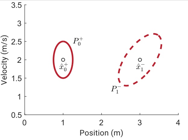
As shown in Figure 2.13a, during propagation the uncertainties in the state covariance matrix grow due to the added uncertainty from the system noise covariance matrix. Based on the strong correlation between velocity and position in this particular example, the shape of the $1\text{-}\sigma$ ellipse also skewed to account for the fact that an uncertainty in velocity at $t_0$ maps to an uncertainty in position at $t_1$. Indeed, the system dynamics (represented by $\Phi$) can generally transform the uncertainty in arbitrary ways.

Update Step

The update step follows the propagation step and combines the prediction of the state vector and state covariance matrix with any available measurement data from the suite of sensors on board a system to provide an optimal estimate of these parameters. The Kalman filter assumes these measurements are valid at an instantaneous time of validity, so timing is critical.

As described in Section 2.7, each of the measurements taken from a sensor is stored in a measurement vector, $\tilde{\boldsymbol{y}}$, and typically requires a conversion prior to being compared to a state. The measurement model matrix, $H$, is used to map the state vector, $\boldsymbol{x}$, into the measurement vector, $\tilde{\boldsymbol{y}}$, as shown in Equation \ref{eq:kfmeasmod}.

\begin{equation} \label{eq:kfmeasmod}\tilde{\boldsymbol{y}}=H\boldsymbol{x} + \boldsymbol{\nu}\end{equation}

Since all sensors produce a measurement with at least some uncertainty (e.g. from noise), the true measured value could actually be a range of possible readings. This uncertainty in each of the measurements is represented by the measurement noise covariance matrix, $R$.

The combination of the measurement model $H$ and the measurement covariance $R$ defines the observability of the system: how well individual states can be estimated (if at all) given those measurements. Low observability translates to large state covariances, and in some cases divergence of the filter if full-state observability is lost for an extended time period.

Once the measurement vector, measurement model matrix, and measurement noise covariance matrix have been formulated, the propagated state vector and state covariance matrix can be combined with this measurement information to provide an updated estimate of the states and state covariance. When combining the measurements with the predictions, a matrix known as the Kalman gain, $K$, is used to weight the measurement information by comparing the uncertainty of the measurement vector ($R$) with the current uncertainty of the state vector ($P$). The Kalman gain is designed such that it is optimal for the system to minimize the variance of the state estimates and can be found using:

\begin{equation} K_{k} = P^{-}_{k}H_{k}^\intercal(H_{k}P^{-}_{k}H_{k}^\intercal + R_{k})^{-1}\end{equation}

To complete the update step, the estimates of the state vector and state covariance matrix are both updated such that:

\begin{equation}\begin{split} \boldsymbol{x}^{+}_{k} &= \boldsymbol{x}^{-}_{k} + K_{k}(\tilde{\boldsymbol{y}}_{k} - H_{k}\boldsymbol{x}^{-}_{k}) \\ P^{+}_{k} &= (I - K_{k}H_{k})P^{-}_{k}\end{split}\label{eq:kfup}\end{equation}

In the aircraft example considered previously, suppose that a sensor is available to measure both position and velocity directly (eg. GPS). The measurement model matrix would then be:

\begin{equation}H = \begin{bmatrix}1&0\\0&1\end{bmatrix}\end{equation}

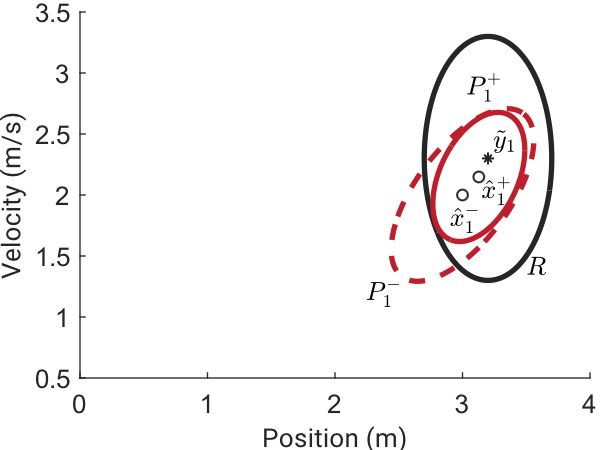
Given the measurement uncertainty $R$ around a noisy measurement $\tilde{\boldsymbol{y}}$, shown in Figure 2.13b, the state and covariance are updated using Equation \ref{eq:kfup}. By incorporating the available measurement data with the prediction of the state vector during the update step, the state covariances in the state covariance matrix shrink as a result of this additional insight into how the system is changing over time.

Tuning a Kalman Filter

Nominally, the terms $Q$ and $R$ represent Gaussian noise that are well-modelled or measured---after all, that is the basis for optimality of a Kalman filter. However, when designing a Kalman filter for a real system, there will always be modelling errors in the propagate step and non-noise-based measurement errors (eg. scale factor errors). To account for these errors and ensure best performance, tuning of the Kalman filter may be required.

Tuning a Kalman filter involves artificially or arbitrarily inflating the system noise covariance matrix, $Q$, as well as the measurement noise covariance matrix, $R$, and in some cases adjusting the initial system covariance matrix, $P_{0}$, as well. These parameters are often referred to as the tuning knobs for the system and must be large enough to maintain enough uncertainty to account for the unmodeled or incorrectly modeled errors, but not too large as unstable behavior could result from the system. The tuning of a Kalman filter is a delicate balancing act that is more of an art than a science. Due to this, tuning is best left to the professionals and is typically performed by the designer of the Kalman filter rather than the end user.