2.10 Feedback Controls

There are two types of controls for dynamic systems: open-loop control and closed-loop (feedback) control. An open-loop system uses only a model of the system without the support of measuring the system response. For example, a conveyor belt that should move at a constant speed may be controlled by setting a constant voltage on the motor which should map to a particular speed given the typical motor and friction of the system. Of course, if the conveyor belt is overloaded, it will move slower than desired and the open-loop controller has no mechanism for correcting it. A closed-loop controller, on the other hand, feeds the measured response of the system back into its control calculations, providing the ability to accurately track the desired output even under varying conditions. For instance, an encoder measuring the turn rate of the conveyor belt would allow a closed-loop controller to maintain the desired speed regardless of loading. Generally, a closed-loop controller measures or estimates an error value, $e(t)$---the difference between the desired state and the measured state---and derives a control input based on that error signal.

Proportional-Integral-Derivative Controller (PID Controller)

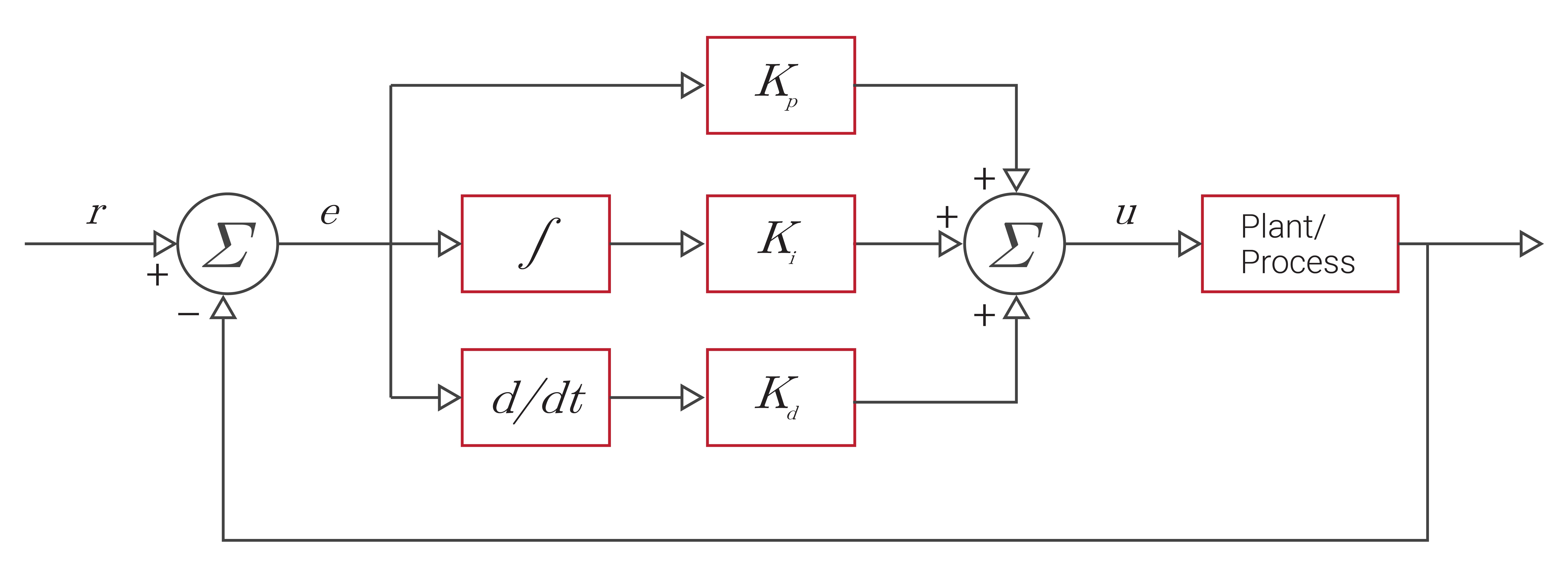
Control systems can be implemented with many different control algorithms, but the vast majority can be characterized as a proportional-integral-derivative (PID) controller. There are three types of control provided by a PID controller based on its namesake: proportional control, integral control, and derivative control. A feedback correction term is then derived using separate gain values from each of the different types of feedback control used in the controller, as illustrated in Figure 2.14. Entire fields of study are devoted to solving for the optimal gains for each of these terms across a wide range of systems.

Proportional

The proportional term (P) applies a multiplier known as the gain, $K_p$, to the value of the direct difference between the measured state and the desired state, as shown in Equation \ref{eq:fcp}. Proportional control is the easiest type of feedback control to implement, though it leads to steady-state errors in a system if used alone.

\begin{equation} \label{eq:fcp}u(t)=K_p * e(t)\end{equation}

Integral

The integral term (I) integrates the error between the desired state and the measured state over time and scales this by a gain value, $K_I$, as shown in Equation \ref{eq:fci}. When used in conjunction with proportional control, this integration acts as a low-pass filter and eliminates the steady-state errors in the system. However, integration of the error can also wind up the controller and lead the system to overshoot the desired value.

\begin{equation} \label{eq:fci}u(t)=K_I \int_0^t e(\tau) \mathrm{d}\tau\end{equation}

Derivative

The derivative term (D) acts on the current rate of change of the error and is scaled by a gain value, $K_D$, as shown in Equation \ref{eq:fcd}. This allows the controller to anticipate the future trend of the error. The more rapid the rate of change of the error, the more impact the derivative controller has on the system. When properly tuned, the derivative term prevents the system from overshooting the desired state.

\begin{equation} \label{eq:fcd}u(t)=K_D\frac{de(t)}{dt}\end{equation}

Each of these feedback correction terms are then summed together and used to calculate an input to the system being controlled, commonly referred to as the plant, to drive the dynamics of the system to the desired state. The individual gain values from each of the different control terms can be tuned to achieve the desired response of the system. Typically, this tuning is performed by the designer of the control system through testing and experimentation.

To visualize how a PID controller works, consider the adaptive cruise control system found commonly in present-day automobiles. Sensors on the automobile take measurements to assess the current conditions of the vehicle and the surrounding environment, such as how fast the automobile is travelling or if another vehicle is approaching. The PID controller then uses this information to derive corrections that will either speed up or slow down the vehicle to achieve the desired speed without overshooting this value.

Latency

In the case of feedback controls, latency is the time delay between when a real-world event occurs and when this data is fed back into the controller. This time delay can cause performance degradation in a system and can even lead to a system becoming unstable or uncontrollable if the latency is longer in duration than the system's time constants. Latency can be at least partially mitigated with appropriate time stamping of the data which informs a controller when the real-world event actually occurred and is commonly referred to as the time of validity of the data. Additionally, lowering the latency in a system, such as by utilizing a real-time operating system, improves the ability to control the system using feedback controls.

Real-Time Operating System (RTOS)

A real-time operating system (RTOS) is a type of operating system (OS) whose purpose is to serve applications needing to process data in real-time with minimal latency. An RTOS has well-defined, fixed time constraints and provides finer controls over priorities and switching behavior between processes. This type of OS also has specialized replacement functions that are re-entrant, meaning that if a process is stopped for whatever reason (e.g. to handle a higher-priority event), the system can re-enter that function and continue where it left off. To minimize latency errors, an RTOS is a crucial component in feedback control systems, which are designed to have fast, low latency feedback responses to ensure proper performance without degradation.

In contrast, the timing on a non-RTOS systems like Windows or standard builds of Linux varies dramatically depending on everything else happening on the system. When timestamping data arriving over a serial port from a sensor, it is not uncommon for the timestamps to vary by 10s or even 100s of milliseconds, despite the data physically arriving at the serial port at a constant rate.