Educational Material
3.4 GNSS Error Budget
The GNSS error budget describes the many factors involved in the GNSS system that determines how accurately a receiver may determine its position, velocity, and time (PVT). Knowledge of these error sources is useful in determining issues that may occur while using a GNSS system. Certain sources of error apply to the individual pseudorange measurements from each satellite, while others can be considered at the level of the PVT solution.
Pseudorange Errors
Table 3.3 provides a list of the various errors impacting individual pseudorange measurements and their impact on those measurements. The total error listed is the result of accumulating those individual errors in a sum-squared sense and represents the typical errors of a standalone GNSS receiver. As discussed in Section 1.5, most receivers track SBAS satellites which provide substantial corrections to each of these terms, bringing the error down to the more commonly seen 2 m specification for consumer GNSS receivers. And more advanced differential GNSS corrections can eliminate some of these errors entirely.
| ERROR SOURCE | ERROR CONTRIBUTION (m RMS) |
|---|---|
| Orbital | 2.5 |
| Satellite Clock | 2 |
| Receiver Noise | 0.3 |
| Ionospheric | 5 |
| Tropospheric | 0.5 |
| Multipath | 1 |
| Total | 11.3 |
Orbit Errors
Any difference between a satellite's actual position and expected position will ripple through the entire PVT determination process. While the ground segment monitors and updates these positions, this still accounts for a large portion of the pseudorange error budget, typically contributing about 2.5 m of error.
Satellite Clock
GNSS trilateration uses the speed of light to measure distances, which means that clock errors are equivalent to range errors. A nanosecond-scale error in the satellite's atomic clock time from relative to GNSS system time results in 0.3 m of pseudorange error and such clock errors typically contribute about 2 m of error.
Receiver Noise
Noise received on the GNSS antenna or from within the receiver itself can contribute a small but not insignificant error to the solution, accounting for around 0.3-1 m of error. Receiver design and antenna quality can significantly impact this error term.
Ionospheric Delay
The ionosphere is the first layer of the atmosphere that a GNSS satellite signal must enter after the vacuum of space, as seen in Figure 3.4. Ranging from 50 km to 1000 km above Earth's surface, the ionosphere contains ionized gases that act as a dispersive medium and slow the propagation speed of radio waves. Since the refractive index is less than one, the signal speed through the medium slows slightly and the phase increases. The ionosphere is also constantly in flux, varying depending on solar activity, time of year, and time of day which therefore cannot be precisely modeled. Due to the many factors involved, ionospheric delay errors can be around 5 m, the largest source of GNSS error.
As mentioned previously, SBAS and other differential GNSS techniques can be used to largely eliminate ionospheric errors. Furthermore, the dispersive nature of the ionosphere causes a higher frequency signal to be slowed less than lower a frequency signal. Due to this, the L1 band experiences less effect than the L2 band, which experiences less than the L5 band. A multi-frequency receiver may use these differences to estimate ionospheric delay directly without external corrections.
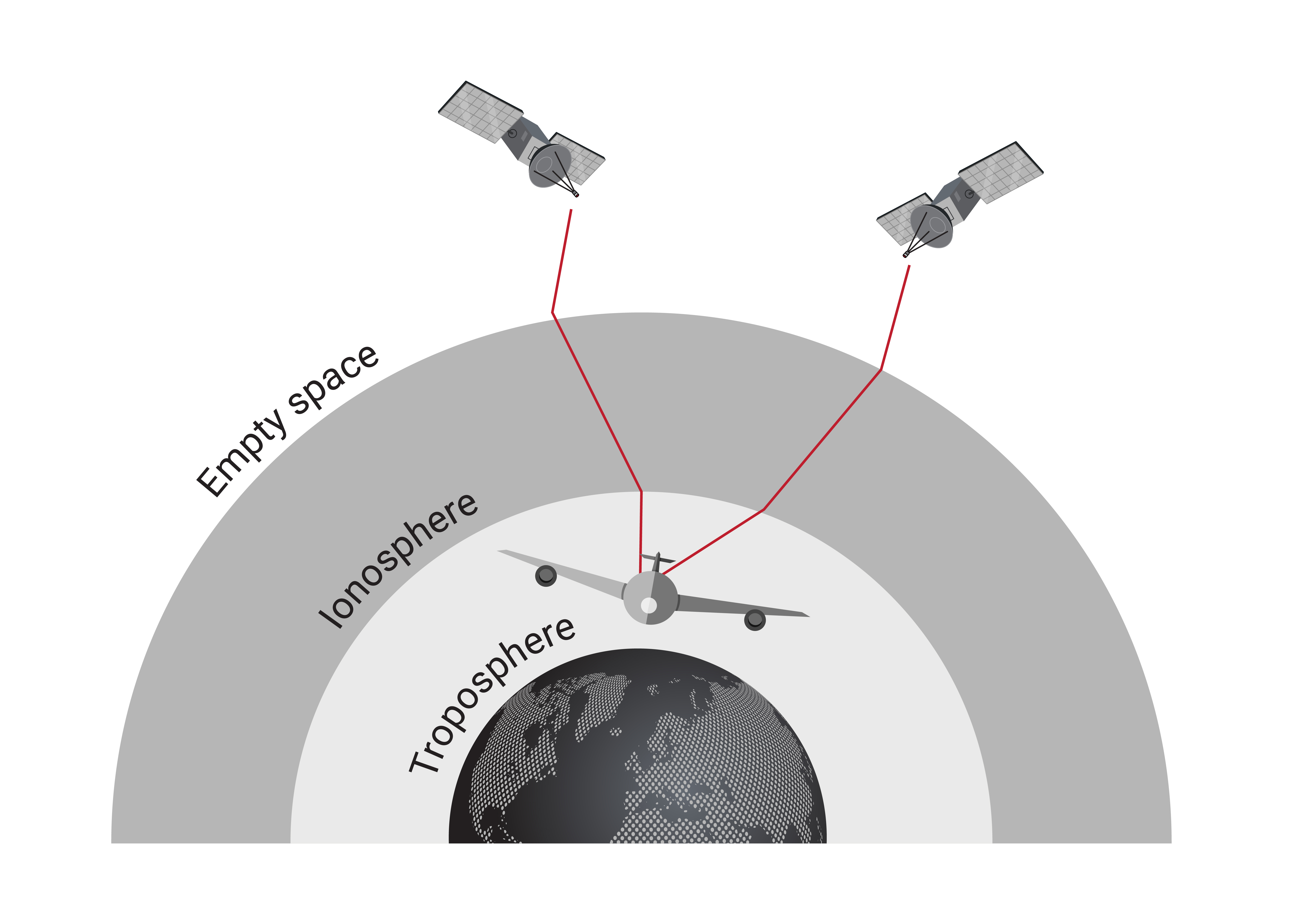
Tropospheric Delay
When a signal enters the troposphere, additional effects come into play affecting signal transmission quality. The troposphere extends from the earth's surface to a height of about 10-16 km, as seen in Figure 3.4. This layer contains all weather on earth, and most of the atmosphere's water vapor. While accurate models exist to predict this delay, changes in pressure, temperature, and humidity still affect signal transmission, resulting in about 0.5 m error.
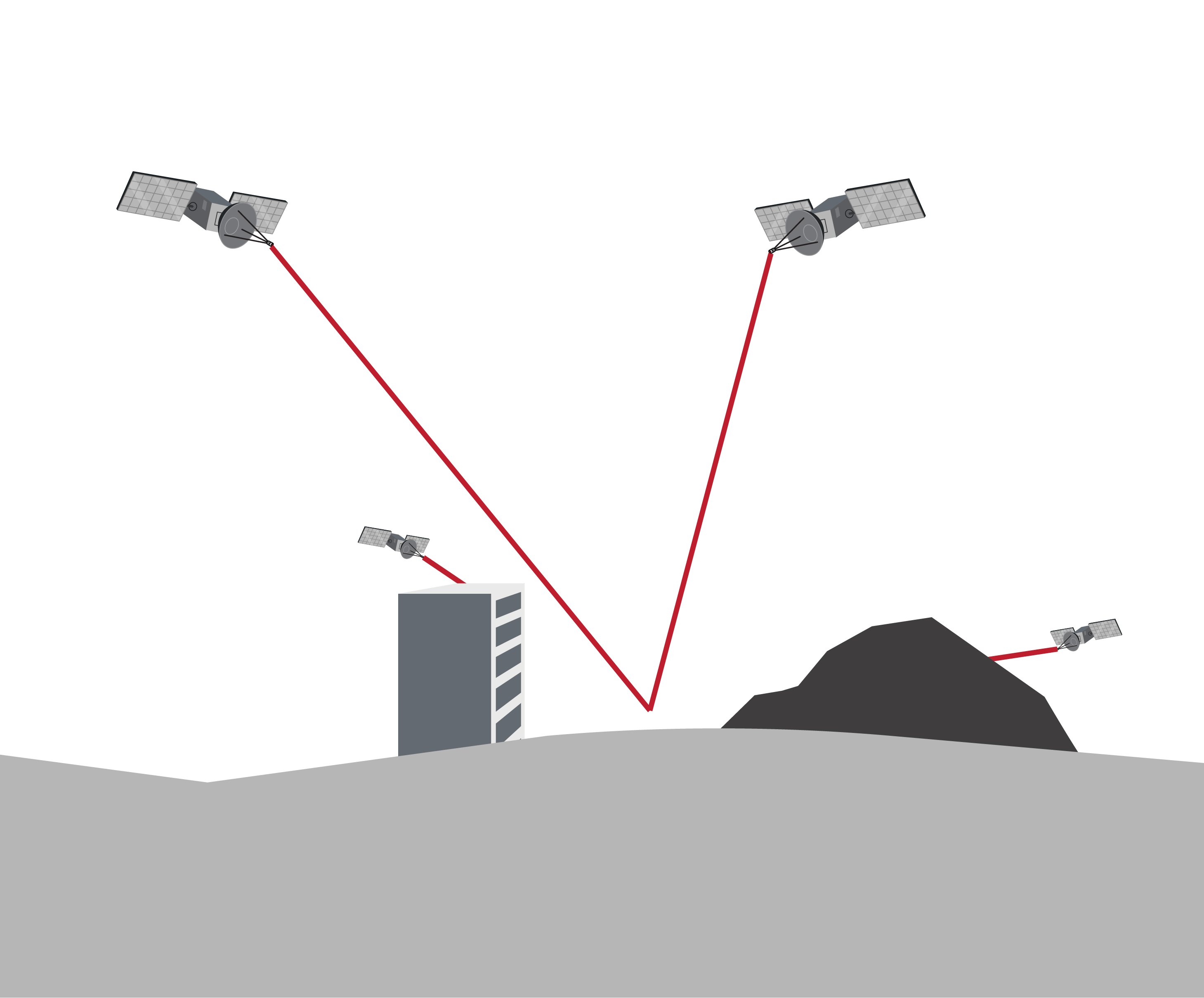
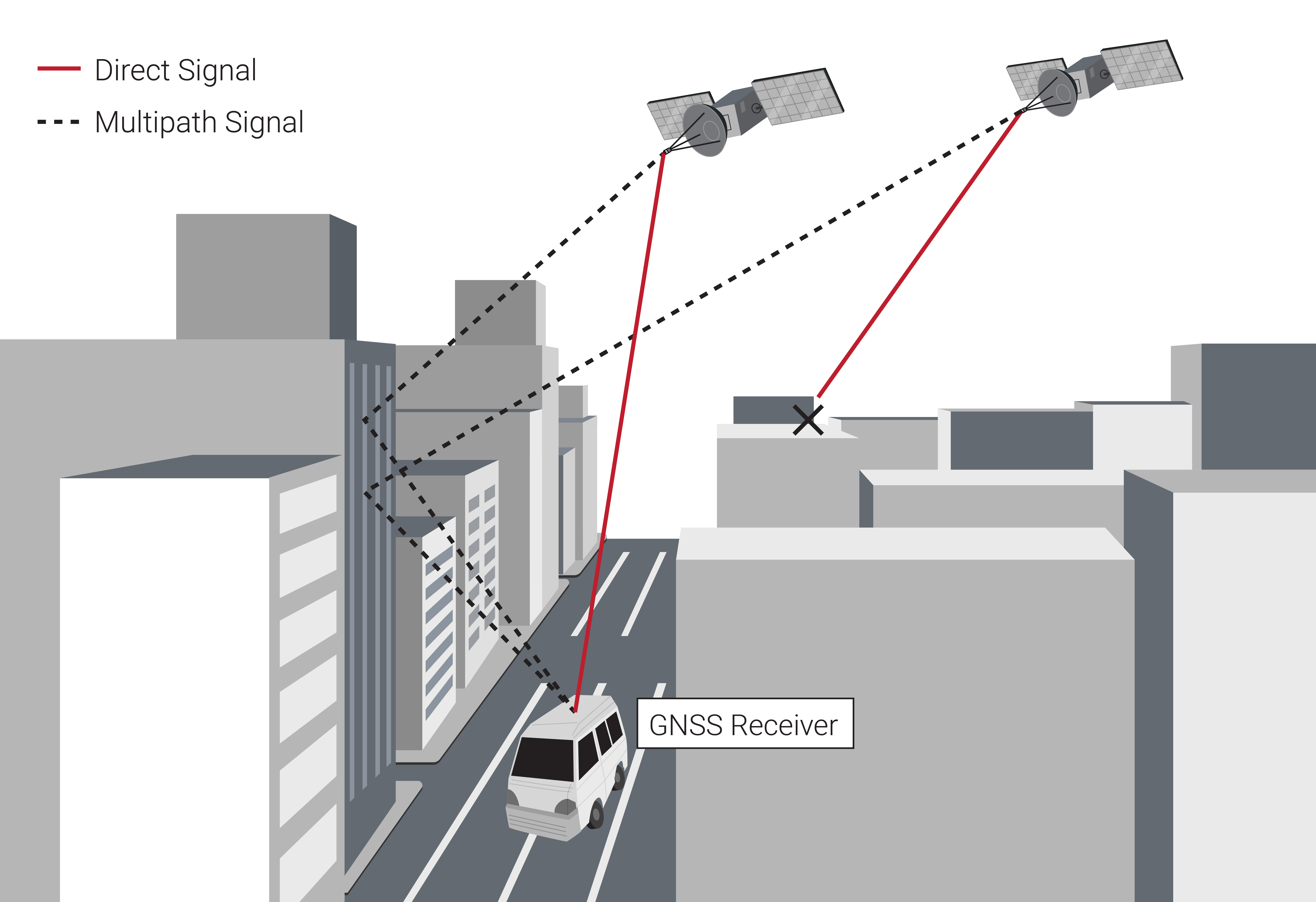
Multipath
Multipath error occurs when GNSS satellite signals bounce off solid objects such as buildings and terrain resulting in the same initial signal taking multiple paths to get to the receiver. This can result in error effects of 1 m or more for the receiver. Figure 3.5 shows some instances of multipath error.
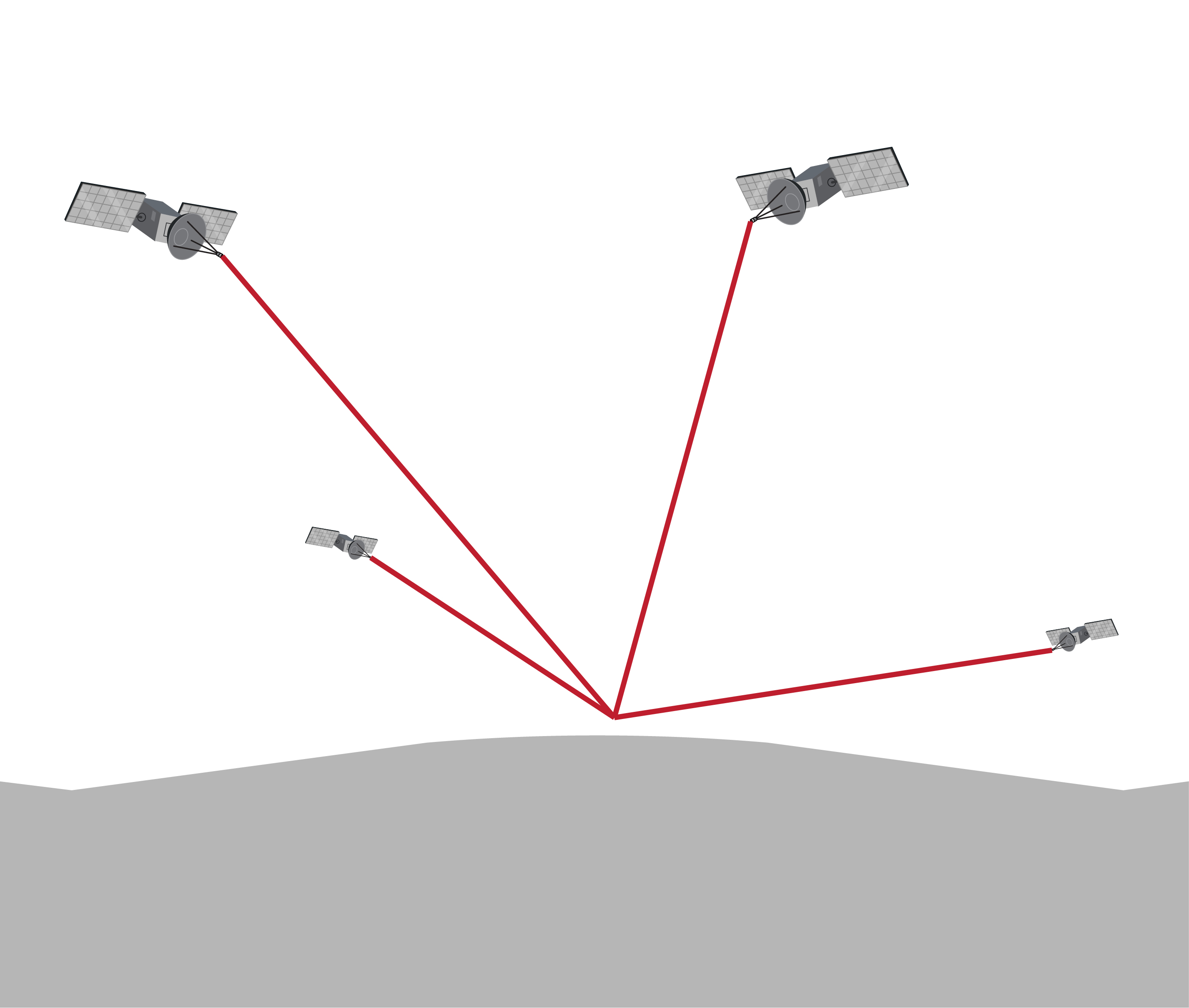
Dilution of Precision
Beyond the errors in the individual pseudoranges, the geometry of the visible (and tracked) satellites contributes to the total PVT error budget. This is known as Dilution of Precision (DOP) and can be calculated in each dimension, including time (since clock errors result in distance errors) and can be combined in a total parameter known as Geometric Dilution of Precision (GDOP). Definitions for the different types of DOP are in Table 3.4.
| DILUTION OF PRECISION | ACRONYM | DEFINITION |
|---|---|---|
| Horizontal | HDOP | $\sqrt{\sigma_{_N}^2+\sigma_{_E}^2}$ |
| Vertical | VDOP | $\sigma_{_D}$ |
| Positional | PDOP | $\sqrt{\mbox{HDOP}^2+\mbox{VDOP}^2}$ |
| Time | TDOP | $\sigma_t$ |
| Geometric | GDOP | $\sqrt{\mbox{PDOP}^2+\mbox{TDOP}^2}$ |
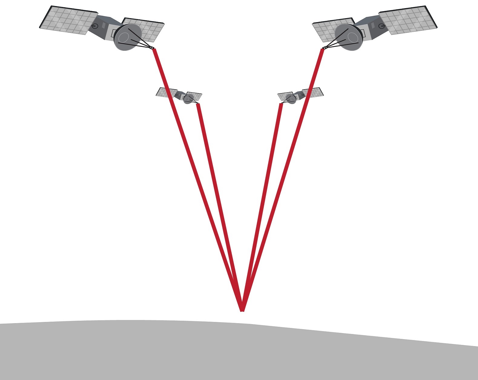
The GDOP represents a sensitivity of the final PVT solution to errors in the pseudoranges. As such, GDOP values are considered ideal when they are low, with values over 5 considered poor. To get a more intuitive understanding of GDOP, the Figure 3.6 contains a few scenarios with varying GDOP. In Figure 3.6a, many well-distributed satellites are visible to the receiver, yielding low GDOP values. Meanwhile, Figure 3.6b shows the visible satellites grouped together overhead, which increases VDOP significantly and, subsequently, high GDOP values. Figure 3.6c contains obstructions that both reduce the number of visible satellites and leave the remaining satellites grouped together, both of which increase GDOP. Increasing the number of available satellites is especially important in this type of scenario, which is why a multi-constellation GNSS receiver is much better suited to urban canyon environments than a GPS-only receiver.