3.1 IMU Specifications

Physical limitations constrain the operation of IMUs in certain applications. A wide variety of standard specifications, and the performance which they describe, should be reviewed to ensure the selection of an appropriate IMU to meet application requirements.

Common Specifications

Range

The range is defined as the minimum and maximum input values a sensor can measure. Anything outside of the range will not be measured or outputted by the sensor.

Resolution

The most precise unit of measure that can be outputted over a sensor's range is known as the resolution. Generally, this specification is not particularly important as most sensors used today have high resolution.

Bandwidth

The bandwidth is the maximum frequency to which a sensor or system will respond. This frequency is typically defined at the point where the response has dropped to half power, or the -3 dB point on a Bode magnitude plot. Bandwidth not only defines the frequencies a sensor can measure, it is inversely related to the time constant of the analog sensor response. Higher bandwidth sensors react more quickly to a given stimulus, and this rise time is the first component in calculating a total system latency.

Sample Rate

Sample rate is the number of samples output by a sensor per second. While sometimes used interchangeably with bandwidth, the sample rate differs as it can be any specified rate while the bandwidth is dependent upon the sensor or system response.

Noise

Noise is classified as any random variation of a measured output when a sensor is subjected to constant input at constant conditions and is usually characterized by either a standard deviation value or a root-mean-square (RMS) value.

Noise Density

Averaging a noisy signal and outputting it at a lower rate, a process known as downsampling, reduces the measured noise of a sensor output. So a single noise standard deviation is insufficient to properly characterize the inherent noisiness of a sensor. While some datasheets will specify that standard deviation at a particular sample rate, the more common measure is noise density which provides the noise divided by the square root of the sampling rate. For example, the noise density for a gyroscope can be represented as $^{\circ}$/s/$\sqrt{\mbox{Hz}}$ or $^{\circ}$/hr/$\sqrt{\mbox{Hz}}$. By multiplying the noise density (ND) by the square root of the sampling rate (SR), the noise standard deviation ($\sigma$) at that rate can be recovered ($\sigma = \mbox{ND}\sqrt{\mbox{SR}}$). Sometimes noise density is specified as a power spectral density, which is simply the noise density squared. In the case of a gyroscope, this yields units of $(^{\circ}/\mbox{s})^2$/Hz.

Random Walk

If a noisy output signal from a sensor is integrated, for example integrating an angular rate signal to determine an angle, the integration will drift over time due to the noise. This drift is called random walk, as it will appear that the integration is taking random steps from one sample to the next. The two main types of random walk for inertial sensors are referred to as angle random walk (ARW), which is applicable to gyroscopes, and velocity random walk (VRW), which is applicable to accelerometers. The specification for random walk is typically given in units of $^{\circ}$/$\sqrt{\mbox{s}}$ or $^{\circ}$/$\sqrt{\mbox{hr}}$ for gyroscopes, and m/s/$\sqrt{\mbox{s}}$ or m/s/$\sqrt{\mbox{hr}}$ for accelerometers. By multiplying the random walk by the square root of time, the standard deviation of the drift due to noise can be recovered.

Unit Conversions

Given three different ways to specify noise (standard deviation at rate, noise density, random walk) and multiple different sets of units used to specify each, it is important to understand how to convert all of them into a common form to get an accurate comparison of different sensors. This mostly requires comfort in performing unit conversions. Section 6.2 works through a number of examples, but here are a few relationships that are particularly useful.

First, it is important to realize that Hertz (Hz) is defined as the inverse of seconds, which means that a noise density specification of $X^{\circ}$/s/$\sqrt{\mbox{Hz}}$ is exactly equivalent to an angle random walk specification of $X^{\circ}$/$\sqrt{\mbox{s}}$ with no conversion necessary.

Second, when working with the square root of time, converting between hours and seconds is a factor of 60 instead of 3600: $60\sqrt{\mbox{s}} = \sqrt{\mbox{hr}}$. So an angle random walk specification of $X^{\circ}/\sqrt{\mbox{s}}$ is equivalent to a specification of $(60\cdot X) ^{\circ}/\sqrt{\mbox{hr}}$.

Finally, the units used for specifying accelerometers often switch between the SI m/s$^2$ and the more common milli-g (mg) (or even micro-g, $\mu$g). It is useful to remember that 1 mg $\approx$ 0.01m/s$^2$. So a noise density specification of $X$ mg/$\sqrt{\mbox{Hz}}$ is roughly equal to a velocity random walk specification of $(0.01X)$ m/s/$\sqrt{\mbox{s}}$.

Bias

The bias is a constant offset of the output value from the input value. There are many different types of bias parameters that can be measured, including in-run bias stability, turn-on bias stability or repeatability, and bias over temperature.

In-Run Bias Stability OR Bias Instability

The in-run bias stability, or often called the bias instability, is a measure of how the bias will drift during operation over time at a constant temperature. This parameter also represents the best possible accuracy with which a sensor's bias can be estimated. Due to this, in-run bias stability is generally the most critical specification as it gives a floor to how accurately a bias can be measured.

Turn-on Bias Stability OR Bias Repeatability

When a sensor is started up, there is an initial bias present that can fluctuate in value from one turn-on to the next due to thermal, physical, mechanical, and electrical variations between measurements. This change in initial bias at constant conditions (eg. temperature) over the lifetime of the sensor is known as the turn-on bias stability, or is sometimes referred to as bias repeatability. While this initial bias cannot be calibrated during production due to its varying nature, an aided inertial navigation system (eg. GNSS-aided) can estimate this bias after each startup and account for it in the outputted measurements. The turn-on bias stability is most relevant for unaided inertial navigation systems or those performing gyrocompassing.

Bias Temperature Sensitivity

As a sensor is operated in a range of temperatures, the bias may respond differently to each of these temperatures. This parameter is known as bias temperature sensitivity and can be calibrated for after each of these biases are measured over the temperature range. However, this bias can only be measured within the limits of the in-run bias stability.

Scale Factor

Scale factor is a multiplier on a signal that is comprised of a ratio of the output to the input over the measurement range. This factor typically varies over temperature and must be calibrated for over the operational temperature range.

Scale Factor Error (ppm or %)

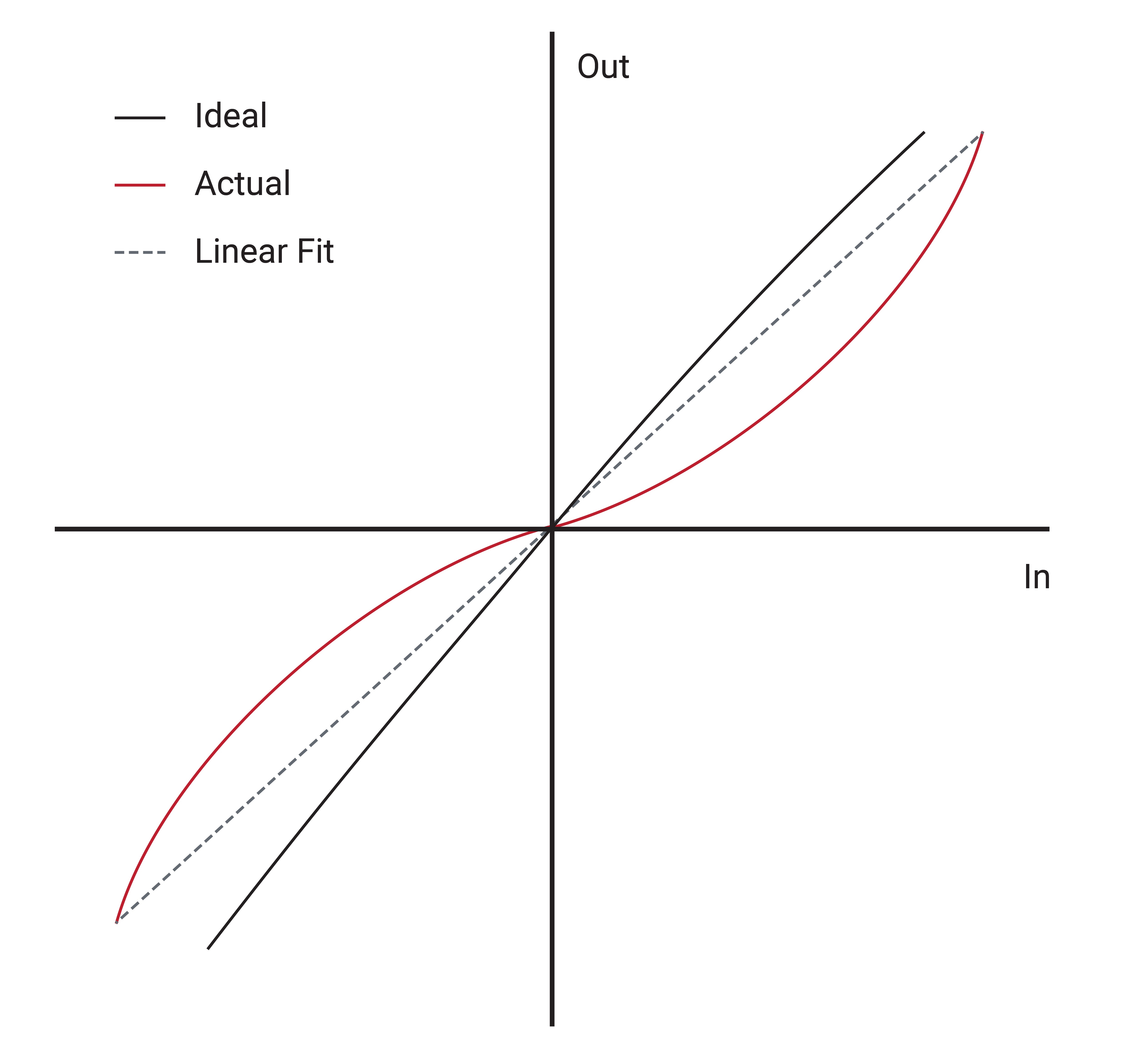
The scale factor will not be perfectly calibrated and will have some error in the estimated ratio. This error is categorized as one of two equivalent values, either as a parts per million error (ppm), or as an error percentage. As shown in Figure 3.1, the scale factor error causes the output reported to be different from the true output. For example, if the z-axis of an accelerometer only measures gravity (9.81 m/s$^2$), then the bias-corrected sensor output should be 9.81 m/s$^2$. However, with a scale factor error of 0.1%, or 1,000 ppm, the output value from the sensor will instead be 9.82 m/s$^2$.

Scale Factor Nonlinearity (ppm or %FS)

The scale factor can also have errors associated with the ratio being non-linear, known as nonlinearity errors, as shown in Figure 3.1. The linearity error of the scale factor is also described as either a parts per million error (ppm), or as a percentage of the full scale range of the sensor.

Orthogonality Errors

When mounting and aligning sensors to an IMU, it is impossible to mount them perfectly orthogonal to each other. As a result, orthogonality errors are caused by a sensor axis responding to an input that should be orthogonal to the sensing direction. The two main types of orthogonality errors are cross-axis sensitivity and misalignment, both of which are often used interchangeably.

Cross-Axis Sensitivity

As defined here, cross-axis sensitivity is an orthogonality error caused by a sensor axis being sensitive to an input on a different axis. In other words, an input in the x-axis may also be partially sensed in the z-axis.

Misalignment

As defined here, misalignment is an orthogonality error resulting from a rigid-body rotation that offsets all axes relative to the expected input axes, while maintaining strict orthogonality between the sensing axes (x-axis remains orthogonal to y- and z-axes). In other words, the internal sensing axes do not align to the axes marked on the case of the IMU. Such misalignment errors exist throughout a full system (e.g. the IMU case is not mounted perfectly aligned to the vehicle, the camera lens is not perfectly aligned to the camera case, etc.). So most high-performance applications require the performance of a separate misalignment calibration across the full end-to-end system (e.g. internal IMU sensing axes to camera lens), and the factory-calibrated misalignment errors of an IMU are largely irrelevant.

Acceleration Sensitivity for Gyroscopes

In an ideal world, a gyroscope would only measure angular rate and would have no sensitivity to linear acceleration. However, in practice gyroscopes are susceptible to linear accelerations due to their asymmetrical design and manufacturing tolerances. The two types of linear acceleration sensitivities are referred to as $g$-sensitivity and $g^2$-sensitivity.

$g$-Sensitivity

An acceleration sensitivity in which a gyroscope experiences a bias shift when subjected to a constant linear acceleration is known as a $g$-sensitivity. Gyroscopes must be tested for sensitivity to linear accelerations both parallel and perpendicular to the sensing axis.

$g^2$-Sensitivity OR Vibration Rectification

The $g^2$-sensitivity specification is an acceleration sensitivity that causes a bias shift in the output of a gyroscope due to oscillatory linear accelerations. As with $g$-sensitivity, gyroscopes must be tested for sensitivity to linear accelerations both parallel and perpendicular to the sensing axis.