3.6 Magnetometer Hard & Soft Iron Calibration

A magnetometer is a sensor used to measure the strength and direction of the local magnetic field surrounding a system. This magnetic field measurement can then be compared to models of Earth's magnetic field to determine the heading of a system with respect to magnetic North. However, in most real-world applications, the magnetic field measured will be a combination of both Earth's magnetic field and magnetic fields created by nearby objects, commonly referred to as magnetic disturbances. In order to obtain an accurate heading estimate, the impact of nearby magnetic disturbances must be mitigated. Internal magnetic disturbances that are non-time varying can be accounted for using a hard & soft iron (HSI) calibration. For more information on magnetic disturbances, refer to Section 3.5.

Magnetometer Sensor Model

In order to mathematically correct sensor measurements for various error sources, a sensor model must be established. As mentioned in Section 3.5, a magnetometer is commonly modeled using the following equation, in which the measurement vector, $\tilde{\boldsymbol{m}}$, consists of a combination of Earth's magnetic field and magnetic fields created by nearby magnetic disturbances.

\begin{equation} \tilde{\boldsymbol{m}} = S_I^{-1}(\boldsymbol{m}_E + \boldsymbol{m}_{e(t)}) + \boldsymbol{b}_{HI} + \boldsymbol{m}_{i(t)}\end{equation}

From this measurement model, a compensation model can be constructed to account for the hard iron, $b_{HI}$, and soft iron, $S_I$, distortions present in the local magnetic field resulting from internal, non-time varying magnetic disturbances.

\begin{equation} \label{eq:magcomp} \boldsymbol{m}_c = S_I(\tilde{\boldsymbol{m}} - \boldsymbol{b}_{HI}) \\\end{equation}

\begin{equation*} \begin{bmatrix} m_{c_x}\\m_{c_y}\\ m_{c_z} \end{bmatrix} = \begin{bmatrix} C_{00} & C_{01} & C_{02} \\ C_{10} & C_{11} & C_{12} \\ C_{20} & C_{21} & C_{22} \end{bmatrix}\begin{bmatrix} \tilde{m}_x - b_{H_0} \\ \tilde{m}_y - b_{H_1} \\ \tilde{m}_z - b_{H_2} \end{bmatrix}\end{equation*}

Hard and Soft Iron Distortions

Magnetic measurements will be subjected to distortion. These distortions are considered to fall in one of two categories: hard iron or soft iron. Hard iron distortions are created by objects that produce a magnetic field. A speaker or piece of magnetized iron for example will cause a hard iron distortion. If the piece of magnetic material is physically attached to the same reference frame as the sensor, then this type of hard iron distortion will cause a permanent bias in the sensor output. Soft iron distortions are considered deflections or alterations in the existing magnetic field. These distortions will stretch or distort the magnetic field depending upon which direction the field acts relative to the sensor. This type of distortion is commonly caused by metals such as nickel and iron. In most cases hard iron distortions will have a much larger contribution to the total uncorrected error than soft iron.

Visualizing Hard and Soft Iron Distortions

A common way of visualizing and correcting hard and soft iron distortions is to plot the output of the magnetometer on a 2D graph. The following examples show measurements taken by the magnetometer as the device is slowly rotated about the z-axis.

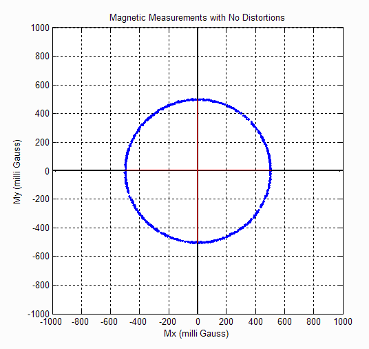
Case 1- No Distortions

In the event that there are no hard or soft iron distortions present, the measurements should form a circle centered at X=0, Y=0, illustrated in Figure 3.7. The radius of the circle equals the magnitude of the magnetic field.

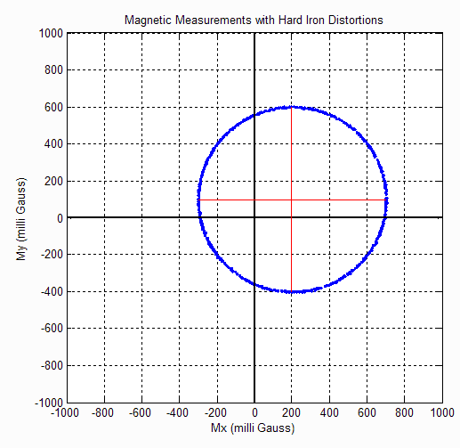
Case 2 - Hard Iron Distortions

Hard iron distortions will cause a permanent bias to be present in the magnetic measurements, which leads to a shift in the center of the circle. As shown in Figure 3.8, the center of the circle is now at X=200, Y=100 with hard iron distortions present. From this it can be concluded that there is 200 mGauss hard iron bias in the X-axis and 100 mGauss hard iron bias in the Y-axis.

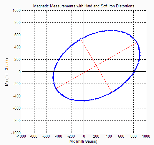
Case 3 - Hard and Soft Iron Distortions

Hard iron distortions will only shift the center of the circle away from the origin, they will not distort the shape of the circle in any way. Soft iron distortions, on the other hand, distort and warp the existing magnetic fields. When plotting the magnetic output, soft iron distortions are easy to recognize as they will distort the circular output into an elliptical shape.

Figure 3.9 illustrates the impact that both hard and soft iron distortions have on the magnetometer output---the circle has been distorted into an ellipse that is not centered at the origin. The center of the ellipse is still located at X=200 and Y=100 since the hard iron distortions are the same as before. Every ellipse has a major and minor axis which corresponds to the long and short dimensions, respectively. As shown in Figure 3.9, the ellipse has its major axis aligned 30° up from the body frame X direction, caused by the soft iron distortions.

Hard and Soft Iron Distortions in 3D Case

While plotting the magnetic measurements on a 2D graph provides a straightforward visualization of the impact of hard and soft iron distortions, in reality the magnetic measurements consist of a full 3D vector. When no distortions are present, the full magnetic measurement vector forms a sphere centered at the origin. Similar to the 2D case, hard iron distortions shift the center of the sphere away from the origin while soft iron distortions distort the sphere into an ellipsoid.

Eliminating Hard and Soft Iron Distortions

It is possible to eliminate the effects of both hard and soft iron distortions on the magnetometer outputs through the use of a hard and soft iron (HSI) calibration. An HSI calibration is a method used to map the biased and distorted ellipsoid back into a sphere centered at the origin. To do so, this calibration is typically implemented with one of two different types of motion, a 2D calibration or a 3D calibration, depending on the range of movement feasible during calibration.

A 2D calibration is generally performed by rotating the magnetometer about the gravity vector in a few 360° circles and is often sufficient if the sensor will stay between 5° to 10° of level in both pitch and roll. Outside of that range, a full 3D calibration is strongly recommended which entails rotating the sensor as much as possible about all axes to cover a sphere of measurement. In either case, hard iron, $\boldsymbol{b}_{HI}$, and soft iron, $S_I$, compensation parameters are estimated from the magnetometer measurements using Equation \ref{eq:magcomp}. For the case shown in Figure 3.9, the corresponding hard and soft iron calibration parameters are shown in Equation \ref{eq:maghsipar}.

\begin{equation}\label{eq:maghsipar} m_c = \left[\begin{matrix} .75 & -.1443 & 0\\ -.1443 & 0.9167 & 0\\ 0 & 0 & 1.0\\ \end{matrix}\right] \left[\begin{matrix} \tilde{m}_x - 0.2\\ \tilde{m}_y - 0.1\\ \tilde{m}_z - 0.0\\ \end{matrix}\right]\end{equation}

The hard iron parameters are set to offset the center of the ellipse by the 200 mGauss in the x-axis and 100 mGauss in the y-axis shown in Figure 3.9 back to the origin. The matrix of soft iron parameters shape the ellipse back into a sphere. Keep in mind, as mentioned previously, that the hard and soft iron distortions influence all axes of the sensor and the above example could be repeated for both rotations about the x- and y- axes.