3.2 IMU Calibration & Characterization

Sensor calibration is a method of improving a sensor's performance by removing structural errors from the measurements of the sensor. Structural errors are differences between a sensor's expected output and its measured output, which show up consistently every time a new measurement is taken. By removing the structural errors, calibration provides a means of improving the overall accuracy of the underlying sensors. These errors are removed through various processes utilizing different equipment and test setups, including rate tables, tumble tests, and thermal chambers.

Sensor characterization incorporates a wide range of tests, including Allan Variance and vibration, to assess the inherent characteristics of the inertial sensors---specifications like noise that cannot be improved through a calibration process. Characterization testing can also be used to verify the post-calibration performance of a sensor to determine parameters such as scale factor error, using the same general testing process used for calibration (though independent of the actual calibration data collection).

Sensor Model

Each sensor is calibrated using the linear sensor model shown in Equation \ref{eq:sensmod}. This equation applies for gyroscopes, accelerometers, and magnetometers. A least-squares fit is performed on the data collected during the calibration process to determine the values of each of the parameters in the model.

\begin{equation}\label{eq:sensmod} \left[\begin{matrix} x\\y\\z\end{matrix}\right] = \left[\begin{matrix} S_x & 0 & 0\\ 0 & S_y & 0\\ 0 & 0 & S_z\end{matrix}\right] \left[\begin{matrix}1 & \alpha_1 & \alpha_2 \\ \alpha_3 & 1 & \alpha_4\\ \alpha_5 & \alpha_6 & 1\end{matrix}\right] \left(\left[\begin{matrix}{\tilde{x}}\\{\tilde{y}}\\{\tilde{z}}\end{matrix}\right] - \left[\begin{matrix}b_x\\b_y\\b_z\end{matrix}\right]\right)\end{equation}

The left-hand side vector is the output from the sensor that has been calibrated for any scale factor errors, misalignment errors, and biases, and should match the truth data after calibration. The two matrices on the right-hand side are known as the scale factor matrix and misalignment matrix, respectively, which contain the sensor's scale factor and misalignment calibration parameters. The scale factor matrix and the misalignment matrix above can also be combined into a single matrix without loss of generality. The last term consists of the uncalibrated measured values and sensor biases. Typically, the biases are the only parameters in the sensor model equation that change significantly over the life of the part and that may require occasional calibration by the user.

Additional terms can be added to the model if they represent significant error sources, including (but not limited to):

• Non-linearity: Rather than a single value for the scale-factor, a polynomial or piece-wise continuous model of the scale factor can be used to address non-linearities across the measurement range.
• g-sensitivity: A gyroscope's bias sensitivity to linear acceleration can be calibrated and used to offset the bias in real time using the measured (and calibrated) accelerometer values.
• Temperature sensitivity: Most calibration parameters in these models have a sensitivity to temperature, so calibrating across the operational temperature range is required. This results in either a look-up table for each of these parameters versus temperature or a polynomial representation.
• Thermal ramp-rate sensitivity: Some advanced sensor calibration models also incorporate a sensitivity to thermal ramp rate, rather than simply assuming a constant temperature.

Calibration Process

Accelerometers are typically calibrated through a process known as a tumble test. During this test, static measurements are taken in different orientations. A tumble test is usually performed by mounting the accelerometer on a cube or a multi-axis turntable that allows each face to be rotated. This exercises the accelerometer by aligning each sensor axis ($X$, $Y$, and $Z$) to the direction of, the direction opposite of, and the directions perpendicular to known gravity as it is rotated, providing a $\pm$1 g measurement.

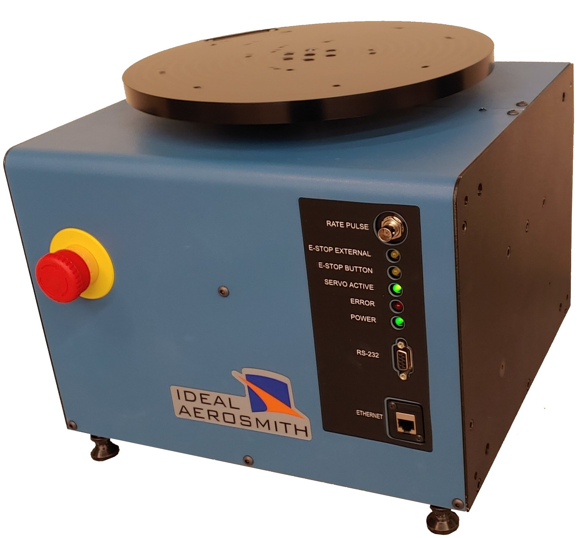
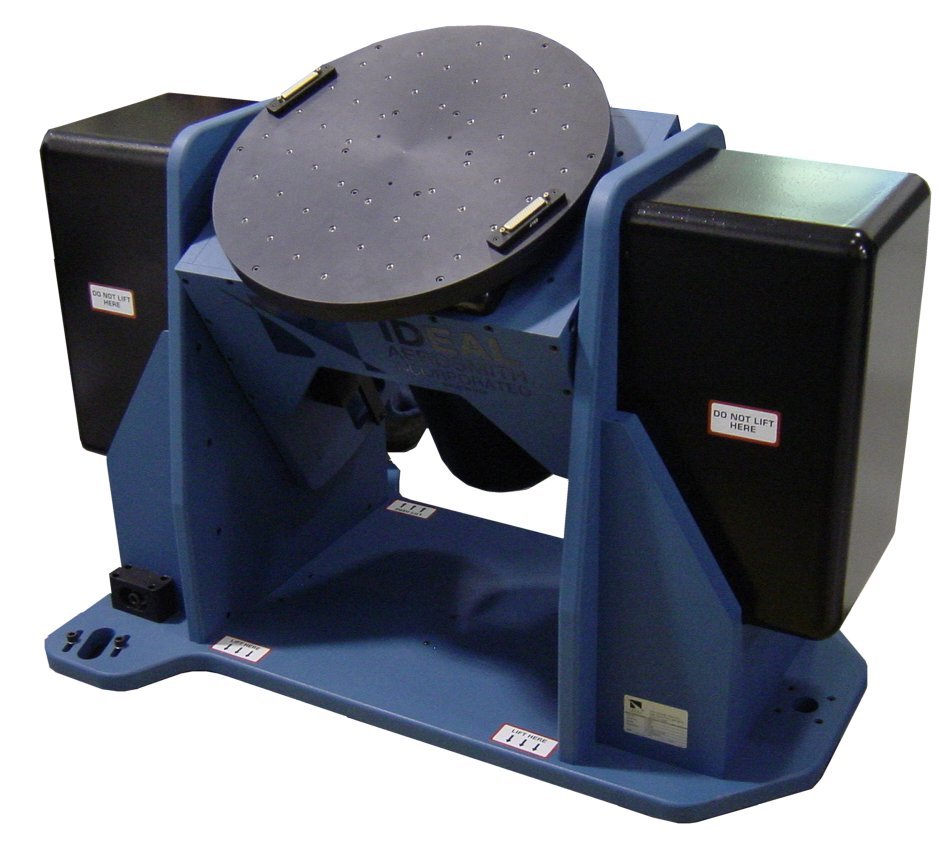
Gyroscopes are calibrated using a precise device known as a rate table. As shown in Figure 3.2a, rate tables have a circular platform connected to a brushless electric motor capable of providing very precise angular and angular rate outputs. The circular rotating platform allows the gyroscope to rotate and be calibrated across a range of angular rates. Rate tables can be purchased as either single-axis (Fig. 3.2a), 2-axis (Fig. 3.2b), or 3-axis systems. A 2-axis system allows for all three gyro axes to be calibrated in a single setup (the tumble test can also be performed), whereas a 3-axis system has the added benefit of being able to reconstruct arbitrary motion profiles.

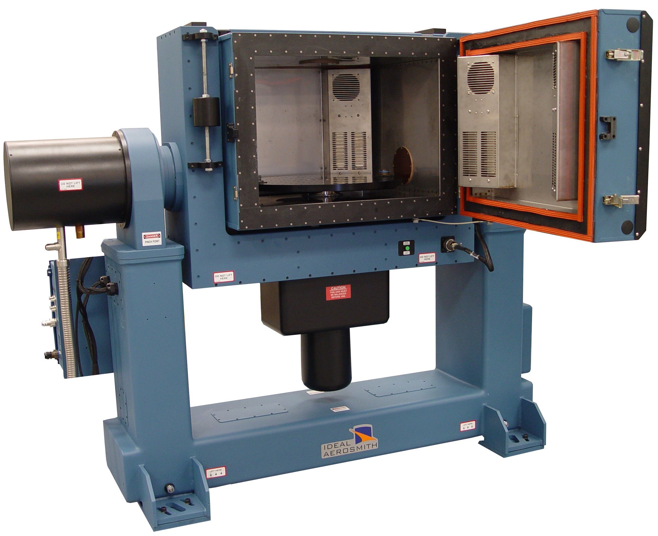
Each of the calibration parameters from the sensor model vary with temperature. A thermal calibration over the sensor's operating temperature range can be performed using a thermal chamber to help mitigate errors due to temperature. As shown in Figure 3.2c, often times a rate table calibration and a tumble test calibration are performed in a temperature controlled thermal chamber to conduct both calibration processes simultaneously.

Allan Variance

An Allan Variance test is a method used for identifying the noise properties of an inertial sensor. A sensor is mounted statically inside a thermal chamber set to a constant temperature, with data logged at high rate for an extended period (typically several hours). The data is downsampled at various time constants (averaged down to lower sampling rates), and the variances of each of these downsampled measurements can be calculated at each of the different time constants. Despite its name, most of the time the results are plotted as standard deviations (square root of variance) versus the downsampled time constants on a log-log scale, as seen in Figure 3.3.

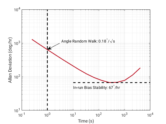
The plot shown in Figure 3.3 illustrates two key specifications for an inertial sensor: (a) the Angle Random Walk (equivalent to noise density, see Section 3.1), and (b) the in-run bias stability. Noise density is roughly equal to the standard deviation at an averaging time constant of one second, while the minimum standard deviation value on the plot is the in-run bias stability.

Vibration Testing

While most calibration processes and characterization tests used to double-check the performance of those parameters utilize steady-state motion, vibration testing allows for the characterization of sensor response relative to time-varying inputs. Typically, a single-axis shaker table is used, requiring the test to be run multiple times to excite all axes. In addition to identifying any unexpected response a sensor may have to vibrations at particular levels or frequencies, vibration testing can be used to determine a number of sensor specifications including:

• Bandwidth: By performing a test known as a sine-sweep---inducing single-frequency vibrations across a range of frequencies---the sensor bandwidth can be determined by finding the frequency associated with the -3 dB point on the response.
• g-sensitivity & g$^2$-sensitivity: Gyroscopes' sensitivity to acceleration can be readily determined through vibration testing, both using sine-sweeps and more general random vibration profiles.