5.4 Relative Localization

Relative localization does not provide information about the global position of the system, but instead provides information relative to the surrounding environment. Consequently, the position error of the system is no longer bounded using such techniques and, given a sufficient amount of time, will often increase beyond acceptable limits for a given application. This section highlights a few techniques that can be used to slow the accumulation of errors in the navigation solution. This list is not meant to be comprehensive or an implementation guide but is meant to provide insight into different approaches can be used.

Free-Inertial Navigation

Free-inertial navigation, sometimes referred to as dead-reckoning, is a classical technique used to estimate a system's position, velocity, and orientation. In such an approach, an inertial navigation system (INS) integrates acceleration and angular rate measurements from an inertial measurement unit (IMU) to track the change in the position, velocity, and orientation of a system.

Often an INS incorporates absolute localization measurements, such as from GNSS or alternative techniques discussed in Section 5.3, into its advanced Kalman filtering algorithms, allowing for a drift-free navigation solution that is tied to an absolute inertial reference frame. Absent such aiding, an INS can only provide a relative navigation solution of how a system changes over time with respect to some initial starting point. Unfortunately, due to a variety of error sources within the inertial sensors themselves (e.g. bias, random walk, etc.), a free-inertial navigation solution will be subject to drift that accumulates exponentially over time. A more in-depth discussion on inertial sensor errors can be found in Section 3.1 and a detailed error budget for free-inertial navigation is presented in Section 3.3.

Odometry

A variety of technologies can produce an odometry measurement - a measured change in position and/or orientation from one time instant to another. Integrating these odometry measurements produces a navigation solution that drifts as a function of distance travelled. Combining odometry with inertial dead-reckoning can significantly reduce the drift rates of the two individual technologies.

Wheels

Wheeled systems can use wheel encoders to estimate how a system has moved. A wheel encoder has discrete markings at evenly spaced angular distances that the encoder can detect and determine the angle the wheel has turned. If the radii of the wheels are known, the angular distance can be converted into a change in position and heading assuming there is no wheel slip. Wheel odometry can be significantly improved by combining it with a gyro measuring heading rate, which can compensate for errors in parameters like wheel radius and help detect wheel slip.

Unlike free-inertial navigation, the accuracy of wheel odometry is dependent on the environment, not on time. In conditions where wheel slip is prevalent, wheel odometry does not produce accurate estimates of the vehicle's motion because the wheel is spinning but not moving. Additionally, wheel odometry is often limited to planar motion and cannot detect changes in elevation, roll, or pitch.

Visual

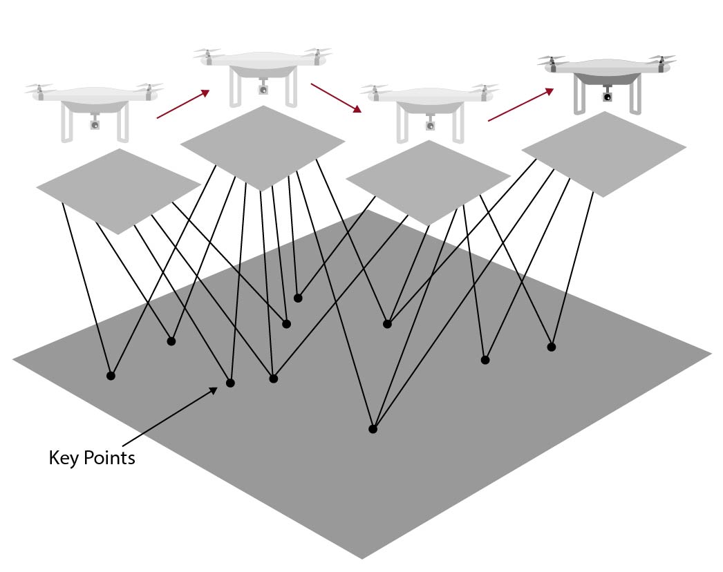
Cameras have become a popular sensor to pair with an IMU for GNSS-denied environments due to their small size, weight, and power consumption (SWaP). Computer vision algorithms enable a computer to track features in an image over time across several image frames and estimate how the camera has moved, as shown in Figure 5.9. When used in conjunction with an IMU, this technique is known as visual-inertial odometry. In the absence of a feature map, no information is available about the global position of the camera—only the motion of the camera relative to the features is measured.

While visual-inertial odometry is attractive for many systems, not all applications are well-suited to navigate with this technique. In order to identify and track unique features within the camera images, there must be sufficient textural variation in the surrounding environment. Applications navigating in areas without such variation, including flying over large bodies of water, often lack unique features needed for visual odometry. The lighting conditions can also affect the quality of a visual odometry solution. A dark environment, such as at night, can prove difficult for an RGB camera and might require an IR camera for successful navigation.

LIDAR

Light Detection and Ranging (LIDAR) has become a popular measurement technique for aiding an IMU in GNSS-denied environments, an approach known as LIDAR-inertial odometry. A LIDAR sensor emits light pulses and times the round trip to measure the distance to reflective objects. Typically, tens or hundreds of thousands of measurements are taken per second, providing the capability to digitize an entire scene almost instantly. This produces a point cloud that can be compared with point clouds from previous scans to track features over time, similar to the visual-inertial odometry technique shown in Figure 5.9. Algorithms such as iterative closest point (ICP) are often used to align the point clouds and determine how the sensor has moved between scans.

While LIDAR sensors provide a dense representation of the surrounding environment, they are not well suited for all applications. Environments that are geometrically uniform, such as a long, straight hallway, prove difficult for navigating using LIDAR-inertial odometry as often there is not a single unique way to align the point clouds measured at two different points. LIDAR sensors are also often heavier and have higher power consumption than other sensors in addition to having a higher cost, making them impractical for some SWaP constrained systems.

Velocity Measurements

Certain technologies can be used to measure linear velocity directly, helping reduce integrated position drift. Unlike odometry, these systems typically do not provide any angular rate feedback to stabilize heading, a major error source in long-term position drift.

Airspeed

Aircraft are often equipped with a pitot tube that is capable of measuring both the static and total air pressure. Differencing these two quantities produces the dynamic air pressure or the pressure due to the motion of the vehicle. The dynamic pressure can be converted into an airspeed measurement that describes the speed of the vehicle with respect to the surrounding body of air. This is different from the ground speed, which is the speed of the vehicle with respect to the ground, as the ground is stationary while the surrounding air can be moving. When the surrounding air is still (i.e. no wind) the two quantities will be equal.

Incorporating airspeed measurements with inertial dead-reckoning, often referred to as airspeed aiding, can be useful in GNSS-denied scenarios because of its ability to provide corrections to the velocity estimate and thus slow the growth of error in the position estimates. For these measurements to be effective, an estimate of the velocity of the surrounding air (i.e. wind speed) must be available to calculate the correct ground speed or the resulting estimates will become biased. Since real-time data about the wind speed in any given location is not readily available it must be estimated in real time.

Doppler Velocity Log

Marine vessels are often equipped with an acoustic sensor called a Doppler Velocity Log (DVL) that sends acoustic pulses toward the sea floor and can measure the velocity of the vehicle by observing the frequency shift of the pulse. A DVL is often used with an IMU or INS to maintain an accurate velocity estimate of an underwater vehicle. Sadly, having an accurate velocity estimate does not mean that the position estimates stays accurate. Small errors in the velocity combined with heading errors translates into large position errors when integrated over a long period of time.

DVL requires operating within a certain range of the seafloor. This range is dependent on the frequency of the DVL pulse—the lower the frequency the longer the range. However, the size and weight of the DVL generally increases as the frequency decreases, requiring a trade-off between operating depth and the size of the sensor.

Simultaneous Localization and Mapping

Simultaneous localization and mapping (SLAM) is a GNSS-denied navigation technique where a user attempts to create a map of an environment and localize themselves using that map. Solving SLAM is traditionally quite challenging as creating a map requires position information but obtaining position information often requires a map in the absence of a GNSS signal resulting in a circular dependency.

SLAM-based navigation utilizes an imager that can capture information about the surrounding environment. Such imagers often include cameras, LiDAR, and radar. Similar to the odometry navigation techniques described previously, features are extracted from the imager data and tracked over time to estimate how the system has moved relative to the features. As additional images are collected, a map of the surrounding environment can be constructed. The biggest difference between SLAM and odometry-based navigation techniques occurs when the navigation system revisits a location that it has already traveled. SLAM systems can identify when a location has been revisited and use this information in a technique called closing the loop. Such loop closures enable SLAM systems to remove large amounts of error from their navigation solution but comes at the cost of more computational complexity.