6.3 Least Squares

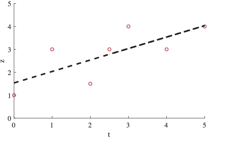
To better understand the linear least squares estimation process described in Section 2.7, consider the collection of data points plotted in Figure 6.1. Each of these points can be written as a linear function using Equation \ref{eq:lslbf}.

\begin{equation} \label{eq:lslbf} z=mt+b\end{equation}

This will form the system of equations shown in Equation \ref{eq:lsese}.

\begin{equation}\label{eq:lsese}\begin{cases}1 &= 0 + b\\ 1.5 &= 2m+b \\4 &= 3m+b \\3 &= 4m+b \\3 &= 2.5m+b\\4 &= 5m+b \\3 &= m+b \\\end{cases}\end{equation}

As seen in Equation \ref{eq:lsesem}, these equations can also be written into an equivalent form using vectors and matrices.

\begin{equation} \label{eq:lsesem}\begin{bmatrix}1\\ 1.5\\ 4\\3\\3\\4\\3\end{bmatrix}=\begin{bmatrix}0&1\\2&1\\3&1\\4&1\\2.5&1\\5&1\\1&1\end{bmatrix}\begin{bmatrix}m\\b\end{bmatrix}\end{equation}

Though a solution cannot be found to solve this system of equations, the linear least squares estimation technique can be used to estimate a line of best fit for this data. Equation \ref{eq:lsesem} follows the same form as Equation \ref{eq:lsem},

\begin{equation} \label{eq:lsem} \boldsymbol{\tilde{y}}=H\boldsymbol{\hat{x}}\end{equation}

where

\begin{equation*}\boldsymbol{\tilde{y}}=\begin{bmatrix}1\\ 1.5\\ 4\\3\\3\\4\\3\end{bmatrix}\text{,} \;\;H=\begin{bmatrix}0&1\\2&1\\3&1\\4&1\\2.5&1\\5&1\\1&1\end{bmatrix}\text{,}\;\;\boldsymbol{\hat{x}}=\begin{bmatrix}m\\b\end{bmatrix}\end{equation*}

These matrices can then be used in the linear least squares solution to solve for the optimal slope and z-intercept of the line of best fit.

\begin{equation*}\begin{split}\boldsymbol{\hat{x}}&=(H^\intercal H)^{-1}H^\intercal\boldsymbol{\tilde{y}}\\&=\left(\begin{bmatrix}0&2&3&4&2.5&5&1\\1&1&1&1&1&1&1\end{bmatrix}\begin{bmatrix}0&1\\2&1\\3&1\\4&1\\2.5&1\\5&1\\1&1\end{bmatrix}\right)^{-1}\begin{bmatrix}0&2&3&4&2.5&5&1\\1&1&1&1&1&1&1\end{bmatrix}\begin{bmatrix}1\\1.5\\4\\3\\3\\4\\3\end{bmatrix}\\&=\begin{bmatrix}0.5\\1.5\end{bmatrix}\end{split}\end{equation*}

As shown in Figure 6.1, the line of best fit that minimizes the residual errors for this collection of data is given by: $z=0.5t+1.5$