2.7 Least Squares

Least squares estimation is a batch estimation technique used to find a model that closely represents a collection of data and allows for the optimal determination of values or states within a system. This estimation technique can be applied to both linear and nonlinear system and is utilized in many different applications.

Linear Least Squares

Many real-world applications often contain an assortment of sensors that can be used to determine various parameters of interest in the system. These parameters of interest are typically referred to as states and can be anything needing to be tracked in a system, such as the position of a spacecraft or the level of saltwater in an aquarium tank.

Each of the states in a system are stored in a vector known as the state vector, $\boldsymbol{x}$. The assortment of sensors in a system is used to provide insight into what is actually happening in the system and how the system is changing over time. Each sensor yields a measurement which is stored in a vector known as the measurement vector, $\tilde{\boldsymbol{y}}$. However, these measurements often only provide information about a state indirectly and often require some type of conversion before being compared to the state vector. The measurement model matrix, $H$, describes this relationship between the measured values and the state values and is used to map the state vector, $\boldsymbol{x}$, into the measurement vector, $\tilde{\boldsymbol{y}}$, as shown in Equation \ref{eq:lsm}, which also takes into account any noise, $\boldsymbol{\nu}$, in the measurement.

\begin{equation} \label{eq:lsm}\tilde{\boldsymbol{y}}=H\boldsymbol{x} + \boldsymbol{\nu}\end{equation}

Ideally, when estimating a particular state, the error between the true value and the estimated value of the state should be minimized. However, in a real-world system, the true value of a state is never actually known due to various error sources, such as measurement errors and modeling errors. As a result, linear least squares instead seeks to minimize the residual error, or the error between the actual measurements, $\tilde{\boldsymbol{y}}$, and the measurements predicted from the measurement model and the estimated value of the state, $\boldsymbol{\hat{x}}$, as shown in the cost function of Equation \ref{eq:lsre}. In this case, the optimal estimate of the state vector for a particular system is found using Equation \ref{eq:lsest}.

\begin{equation} \begin{split} J &= \frac{1}{2}\sum{\boldsymbol{e}^\intercal\boldsymbol{e}} \\ \boldsymbol{e}&=\tilde{\boldsymbol{y}}-H\boldsymbol{\hat{x}}\end{split}\label{eq:lsre}\end{equation}

\begin{equation} \label{eq:lsest} \boldsymbol{\hat{x}}=(H^\intercal H)^{-1}H^\intercal\tilde{\boldsymbol{y}}\end{equation}

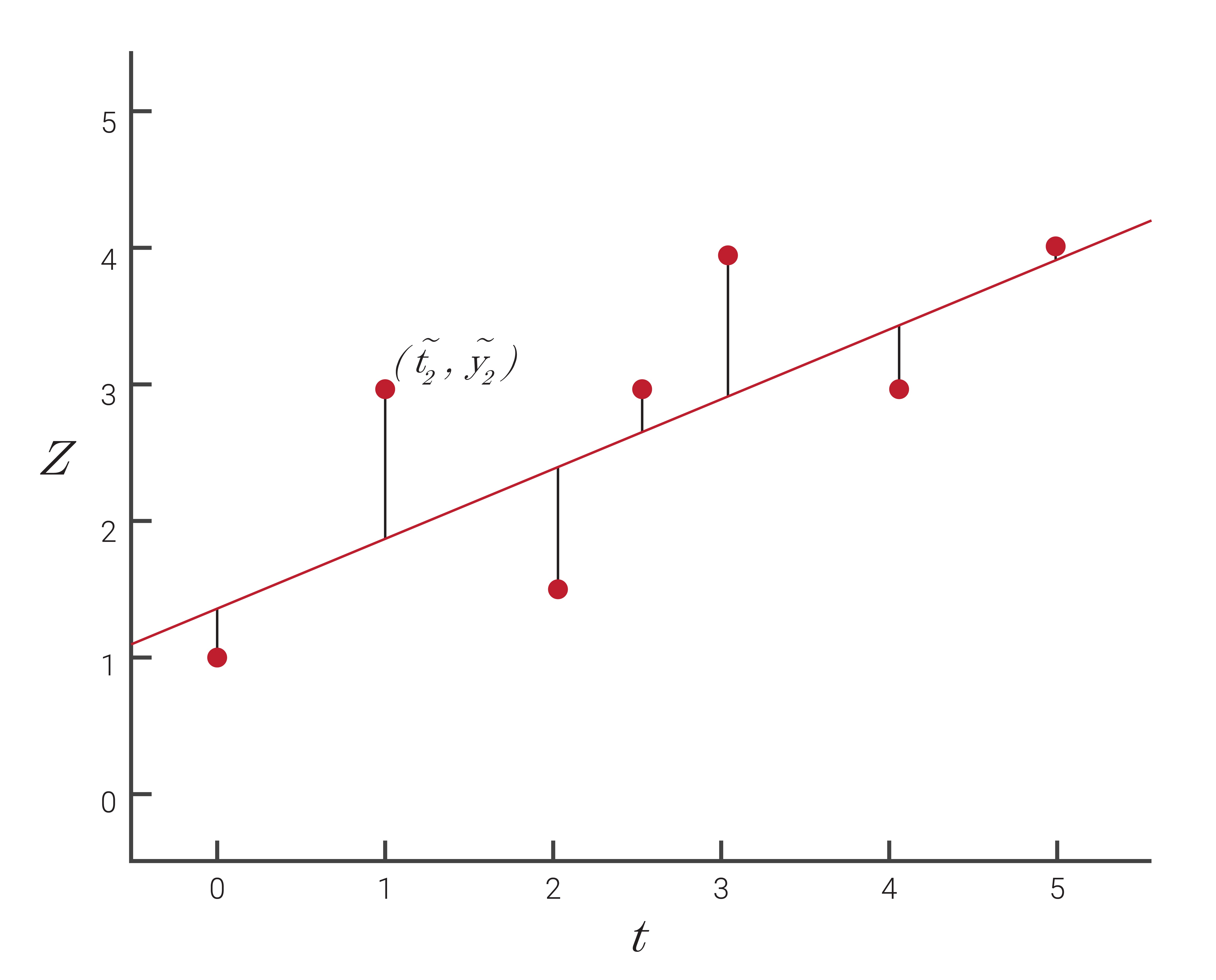
To visualize the linear least squares estimation process, consider the collection of data points plotted in Figure 2.12. While no line exists that can connect all of the data points together, there are a variety of lines that can be used to provide different fits of the data. As shown in detail in Section 6.3, linear least squares determines the line that provides the best fit for this set of data. Though commonly used in curve fitting applications, linear least squares can be used in a variety of other applications as well including identifying the best model for a particular system or determining specific parameters of interest in a system.

Weighted Least Squares

The linear least squares solution determines the optimal estimate for each of the estimated state values by minimizing the residual error while weighing each of the measurements equally. However, many applications utilize numerous sensors that have varying performance specifications and uncertainties. In this case, weighing each measurement equally is not as useful. A technique known as weighted least squares adds an appropriate weight to each measurement to account for the uncertainty in each of the measurements. The linear least squares solution then becomes:

\begin{equation} \boldsymbol{\hat{x}}=(H^\intercal WH)^{-1}H^\intercal W\tilde{\boldsymbol{y}}\end{equation}

where $W$ is a symmetric, positive-definite matrix that contains the appropriate weights for each measurement. While any user-defined weights can be used in $W$, setting this matrix is set equal to the inverse of the measurement covariance matrix, $R$, yields optimal results.

\begin{equation} \boldsymbol{\hat{x}}=(H^\intercal R^{-1}H)^{-1}H^\intercal R^{-1}\tilde{\boldsymbol{y}}\end{equation}

Note that in this case, the $(H^\intercal R^{-1}H)^{-1}$ term in the weighted least squares solution is then equal to the state covariance matrix, $P$.

\begin{equation} P=(H^\intercal R^{-1}H)^{-1}\end{equation}

For more information about the measurement covariance matrix and the state covariance matrix, refer to Section 2.8.

Nonlinear Least Squares

While linear least squares can be used in various applications, some systems cannot be described by a linear model. For these nonlinear systems, the linear least squares solution can be extended to a nonlinear least squares solution, also known as the Gaussian Least Squares Differential Correction (GLSDC). The nonlinear least squares estimation process uses a model of the form:

\begin{equation} \tilde{\boldsymbol{y}}=\boldsymbol{h}(\boldsymbol{x})\end{equation}

where $\boldsymbol{h}(\boldsymbol{x})$ represents the equations of a nonlinear system. An optimal estimate for a nonlinear system can then be found by iterating the nonlinear least squares solution, using Equation \ref{eq;nonlinls}.

\begin{equation}\begin{split} \hat{\boldsymbol{x}}_{k+1} = \hat{\boldsymbol{x}}_{k} + (H_k^\intercal& H_k)^{-1}H_k^\intercal \left(\tilde{\boldsymbol{y}} - \boldsymbol{h}(\hat{\boldsymbol{x}}_k)\right)\\ H_k&=\frac{\delta\boldsymbol{h}}{\delta\hat{\boldsymbol{x}}_k}\end{split}\label{eq;nonlinls}\end{equation}

where the $H$ matrix is known as the Jacobian matrix. Weighted versions of this calculation follow the same formulation as the linear case. Though this iterative process requires more computation than the linear least squares estimation process, nonlinear least squares provides the advantage of optimizing a wide range of real-world systems.